R Graphics メモ
INOUE Takakatsu 最終更新: 2020-09-30
作図
#     par(family="Japan1",mfrow=c(1,1))
#
#     plot(x, y = NULL, type = "p",  xlim = NULL, ylim = NULL,
#          log = "", main = NULL, sub = NULL, xlab = NULL, ylab = NULL,
#          ann = par("ann"), axes = TRUE, frame.plot = axes,
#          panel.first = NULL, panel.last = NULL,
#          col = par("col"), bg = NA, pch = par("pch"),
#          cex = 1, lty = par("lty"), lab = par("lab"),
#          lwd = par("lwd"), asp = NA, ...)
関数の描画 plot
定義域と関数値をそれぞれベクトル x, y で与え, y=f(x)のグラフを作成する.
x <- seq(-pi, 2*pi, length.out=51)                   # 定義域をベクトルで設定
str(x)
## num [1:51] -3.14 -2.95 -2.76 -2.58 -2.39 ...y <- sin(x)
str(y)## num [1:51] -1.22e-16 -1.87e-01 -3.68e-01 -5.36e-01 -6.85e-01 ...plot(x, y, type="l", family="Japan1", xlab="x [ラジアン]", ylab="正弦(sin)関数",
main="fig-1a : 関数プロット1") # 定義域(ベクトル)x, 関数値ベクトルyを指定する場合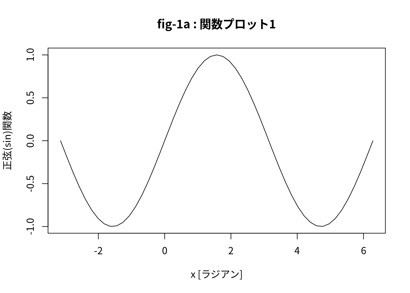
関数名と定義域の下限,上限を与えて関数を描画する.
plot(sin, -pi, 2*pi, family="Japan1", main="fig-1b : 関数プロット2") # 関数名, 定義域の下限, 上限 で指定する場合 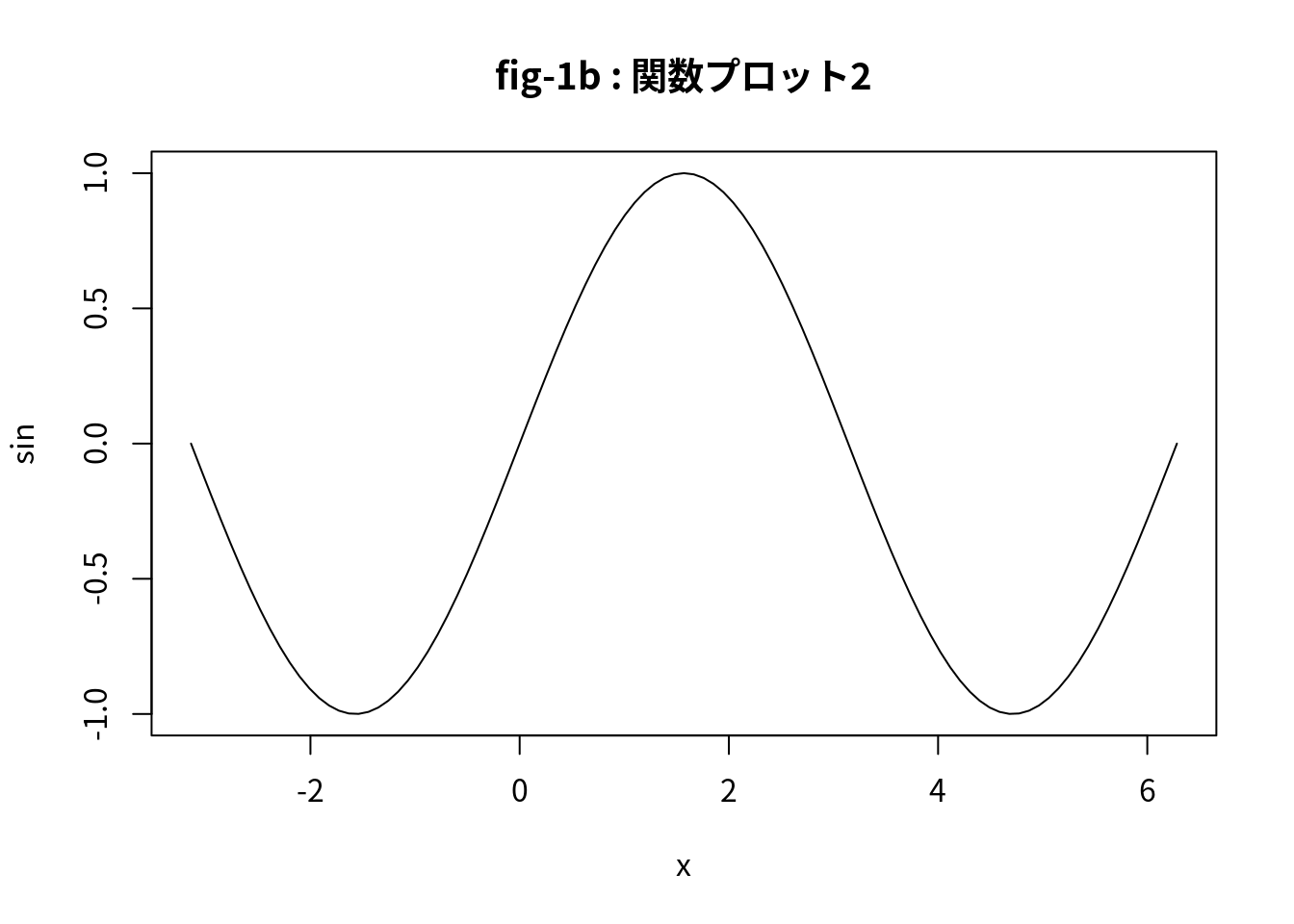
plot, curve による作図
###### example of curve ##############################################
  op <- par(mfrow=c(1,2))
  curve(x^3 - 3 * x, -2, 2, family="Japan1", main="3次,2次式")     # 3次式
  curve(x^2 - 2, add = TRUE, col = "violet")    # 2次式の追加
  plot(cos, xlim = c(-pi, 3 * pi), n = 101,
       col = "blue", family="Japan1", main="余弦曲線")             # コサイン曲線(右図)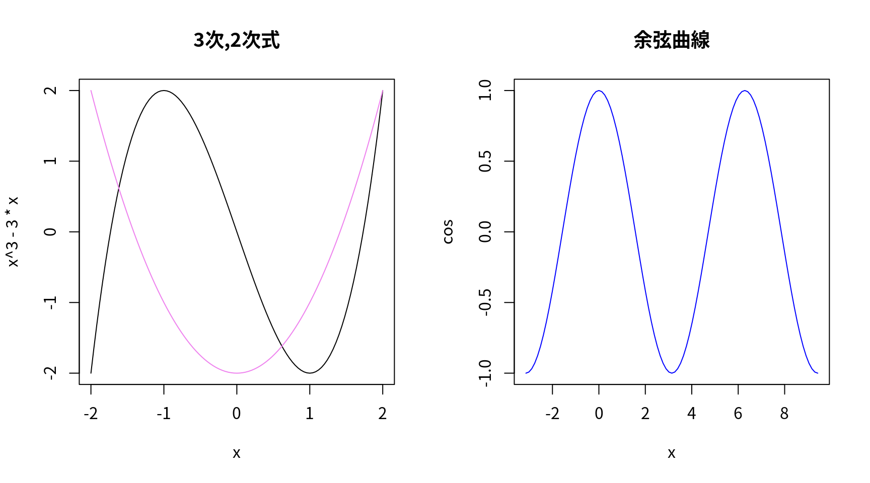
  chippy <- function(x) sin(cos(x) * exp(-x/2)) #関数chippyの定義
  curve(chippy, -8,  7, n=101, main="chippy on [-8,7]")
  curve(chippy, -8, -5, n=101, main="chippy on [-8,-5]")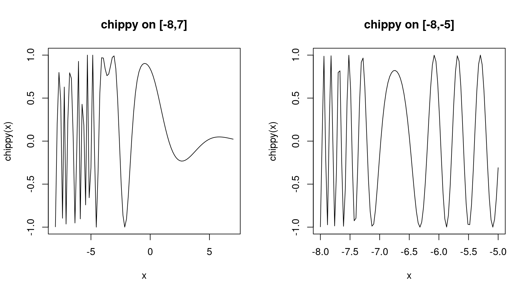
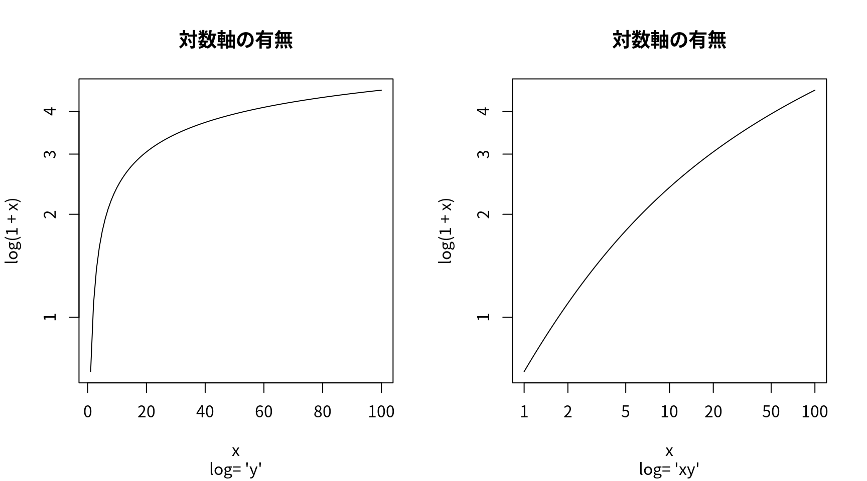
対数軸使用の有無
   op <- par(mfrow = c(1, 2))
   for (ll in c("", "x", "y", "xy")) {
     curve(log(1 + x), 1, 100, log = ll,
           sub = paste("log= '", ll, "'", sep = ""),
           family="Japan1", main="対数軸の有無")
     } # end of for-ll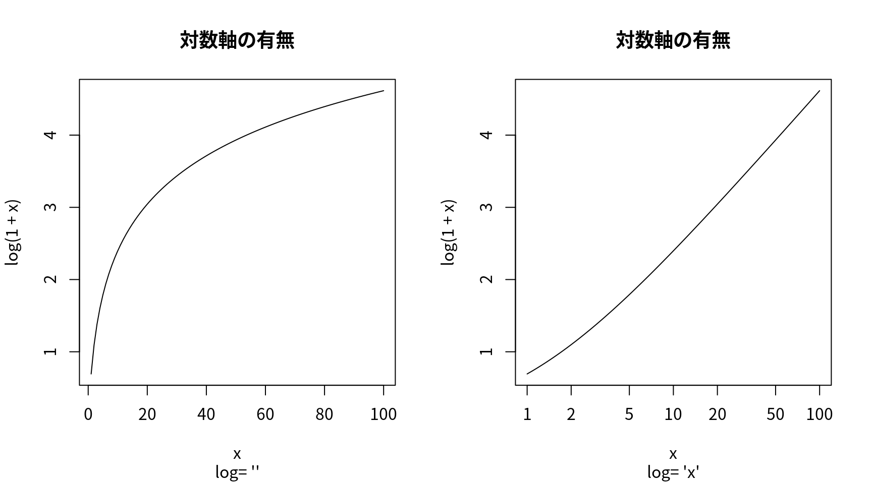
matplot, matpoints, matlines による作図
#     matplot(x, y, type = "p", lty = 1:5, lwd = 1, pch = NULL,
#             col = 1:6, cex = NULL,
#             xlab = NULL, ylab = NULL, xlim = NULL, ylim = NULL,
#             ..., add = FALSE, verbose = getOption("verbose"))
#
#     matpoints(x, y, type = "p", lty = 1:5, lwd = 1, pch = NULL,
#               col = 1:6, ...)
#
#     matlines (x, y, type = "l", lty = 1:5, lwd = 1, pch = NULL,
#               col = 1:6, ...)
###### example of matplot ##############################################
  matplot(-4:4, (-4:4)^2, main = "Fig.21 : Quadratic")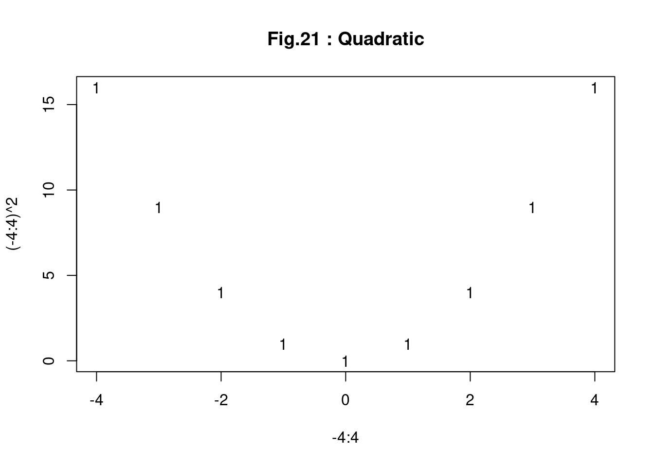
  sines <- outer(0:20, 1:4, function(x, k) sin(x/20 * pi * k))
  sines
## [,1] [,2] [,3] [,4]
## [1,] 0.000000e+00 0.000000e+00 0.000000e+00 0.000000e+00
## [2,] 1.564345e-01 3.090170e-01 4.539905e-01 5.877853e-01
## [3,] 3.090170e-01 5.877853e-01 8.090170e-01 9.510565e-01
## [4,] 4.539905e-01 8.090170e-01 9.876883e-01 9.510565e-01
## [5,] 5.877853e-01 9.510565e-01 9.510565e-01 5.877853e-01
## [6,] 7.071068e-01 1.000000e+00 7.071068e-01 1.224647e-16
## [7,] 8.090170e-01 9.510565e-01 3.090170e-01 -5.877853e-01
## [8,] 8.910065e-01 8.090170e-01 -1.564345e-01 -9.510565e-01
## [9,] 9.510565e-01 5.877853e-01 -5.877853e-01 -9.510565e-01
## [10,] 9.876883e-01 3.090170e-01 -8.910065e-01 -5.877853e-01
## [11,] 1.000000e+00 1.224647e-16 -1.000000e+00 -2.449294e-16
## [12,] 9.876883e-01 -3.090170e-01 -8.910065e-01 5.877853e-01
## [13,] 9.510565e-01 -5.877853e-01 -5.877853e-01 9.510565e-01
## [14,] 8.910065e-01 -8.090170e-01 -1.564345e-01 9.510565e-01
## [15,] 8.090170e-01 -9.510565e-01 3.090170e-01 5.877853e-01
## [16,] 7.071068e-01 -1.000000e+00 7.071068e-01 3.673940e-16
## [17,] 5.877853e-01 -9.510565e-01 9.510565e-01 -5.877853e-01
## [18,] 4.539905e-01 -8.090170e-01 9.876883e-01 -9.510565e-01
## [19,] 3.090170e-01 -5.877853e-01 8.090170e-01 -9.510565e-01
## [20,] 1.564345e-01 -3.090170e-01 4.539905e-01 -5.877853e-01
## [21,] 1.224647e-16 -2.449294e-16 3.673940e-16 -4.898587e-16 str(sines)## num [1:21, 1:4] 0 0.156 0.309 0.454 0.588 ... matplot(sines, pch = 1:4, type = "o", col = rainbow(ncol(sines)),
main = "Fig.22 : sines")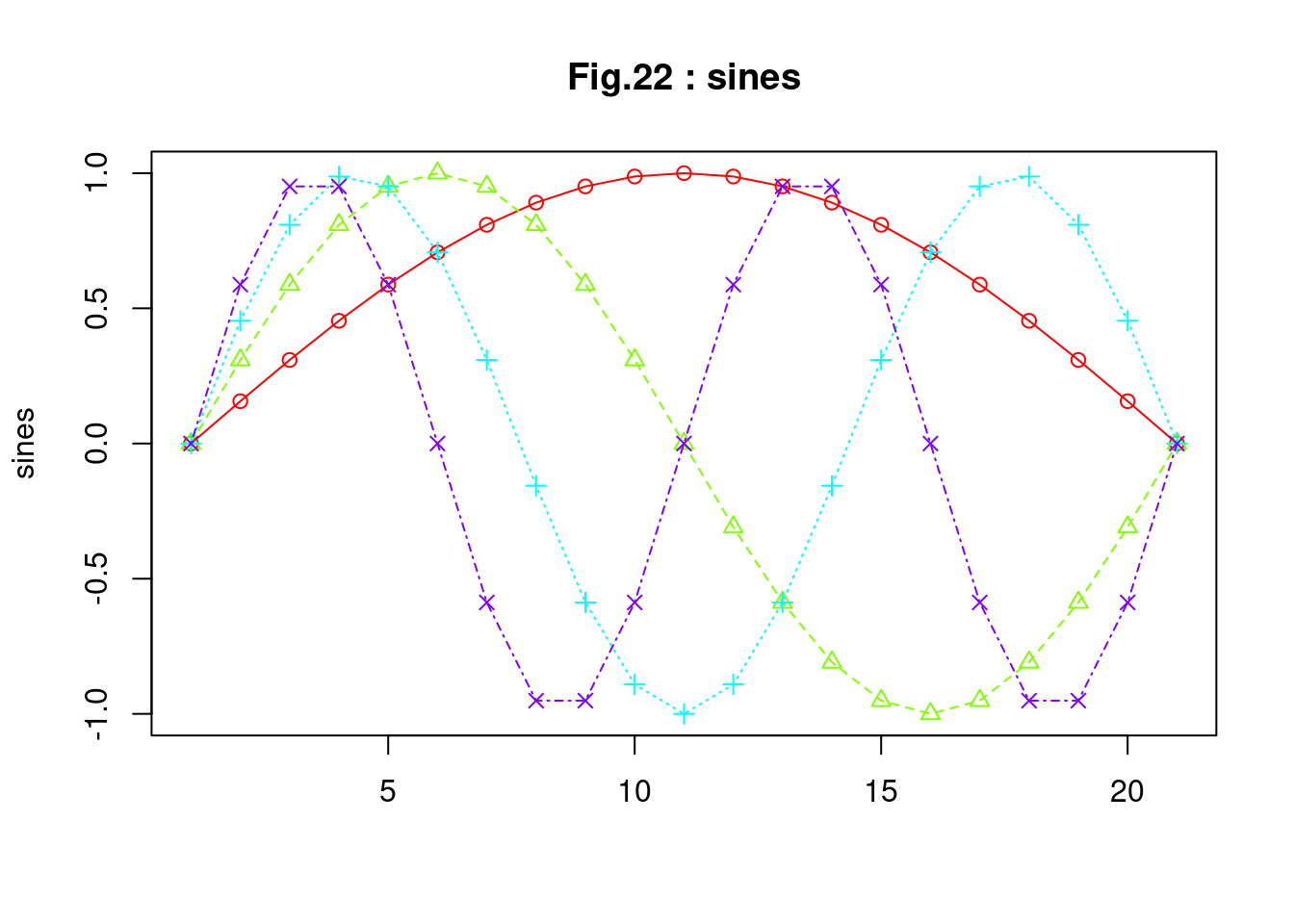
   x <- 0:50/50
   matplot(x, outer(x, 1:8, function(x, k) sin(k * pi * x)),
           ylim = c(-1.5, 1.5), type = "plobcsSh",
           main = "Fig.23 : matplot(,type = \"plobcsSh\" )")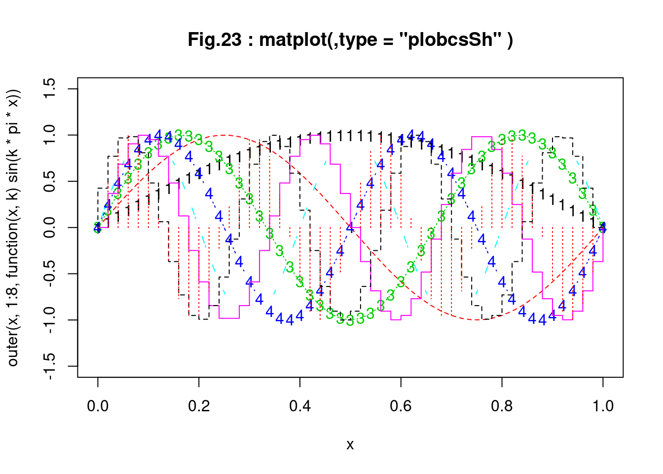
   matplot(x, outer(x, 1:4, function(x, k) sin(k * pi * x)),
           pch = letters[1:4], type = c("b", "p", "o"),
           main = "Fig.24 : matplot(,type = c(\"b\", \"p\", \"o\")")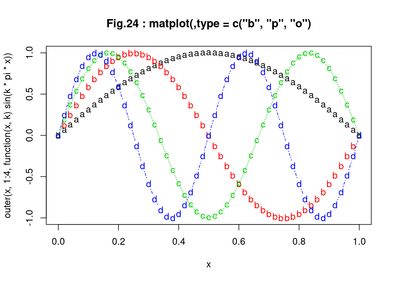
table(iris$Species)##
## setosa versicolor virginica
## 50 50 50 iS <- iris$Species == "setosa"
iV <- iris$Species == "versicolor"
op <- par(cex.main=1.5)
matplot(c(1, 8), c(0, 4.5), type = "n", xlab = "Length", ylab = "Width",
main = "Fig.25 : Petal and Sepal Dimensions in Iris Blossoms")
matpoints(iris[iS, c(1, 3)], iris[iS, c(2, 4)], pch = "sS", col = c(2, 4))
matpoints(iris[iV, c(1, 3)], iris[iV, c(2, 4)], pch = "vV", col = c(2, 4))
legend(1, 4, c("Setosa Petals", "Setosa Sepals", # 凡例
"Versicolor Petals", "Versicolor Sepals"), pch = "sSvV",
col = rep(c(2, 4), 2))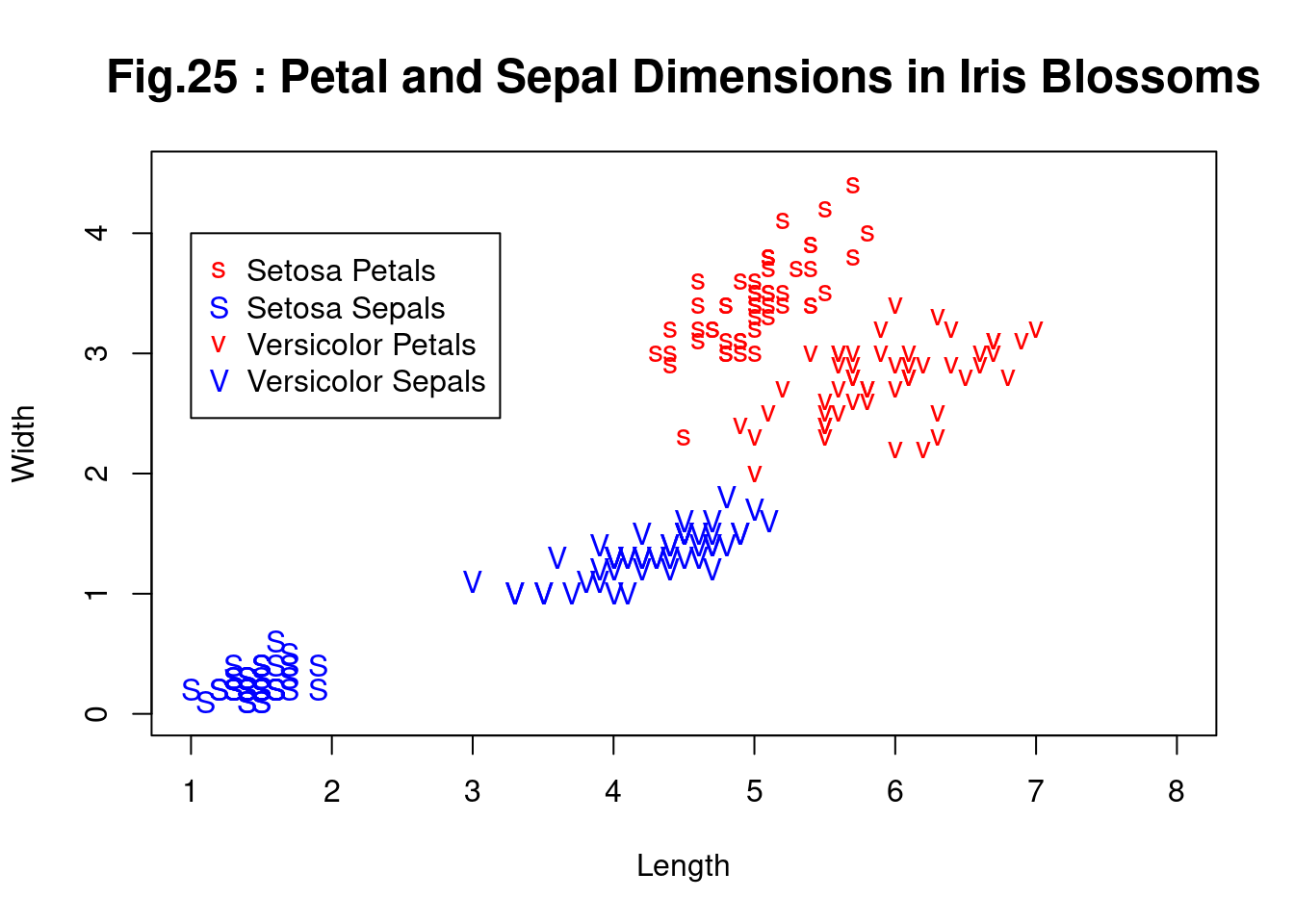
注: iris setosa(ヒオウギアヤメ), iris versicolor(青または青みがかったスミレ色の花を持つ、米国東部のよくあるアヤメ) , Petals(花びら), sepal(がく片),
ヒストグラム
hist
###### example of barplot ##############################################
   tN <- table(Ni <- rpois(100, lambda = 5))  # ポアソン乱数を生成
   str(Ni)
## int [1:100] 3 9 1 7 5 2 6 3 3 5 ... cat("av =",mean(Ni),", var =",var(Ni),", sd =",sqrt(var(Ni)),"\n")## av = 5.18 , var = 4.896566 , sd = 2.212818 tN##
## 1 2 3 4 5 6 7 8 9 10 11
## 3 8 15 15 17 12 12 12 4 1 1 (hist(Ni)) # ヒストグラムの表示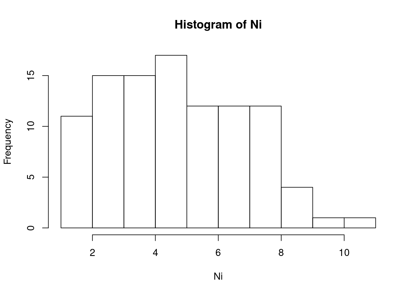
## $breaks
##  [1]  1  2  3  4  5  6  7  8  9 10 11
##
## $counts
##  [1] 11 15 15 17 12 12 12  4  1  1
##
## $density
##  [1] 0.11 0.15 0.15 0.17 0.12 0.12 0.12 0.04 0.01 0.01
##
## $mids
##  [1]  1.5  2.5  3.5  4.5  5.5  6.5  7.5  8.5  9.5 10.5
##
## $xname
## [1] "Ni"
##
## $equidist
## [1] TRUE
##
## attr(,"class")
## [1] "histogram"
r <- barplot(tN, col = "gray", main="Fig.51 : barplot") # バープロット
lines(r, tN, type = "h", col = "red", lwd = 2) # 赤線の追加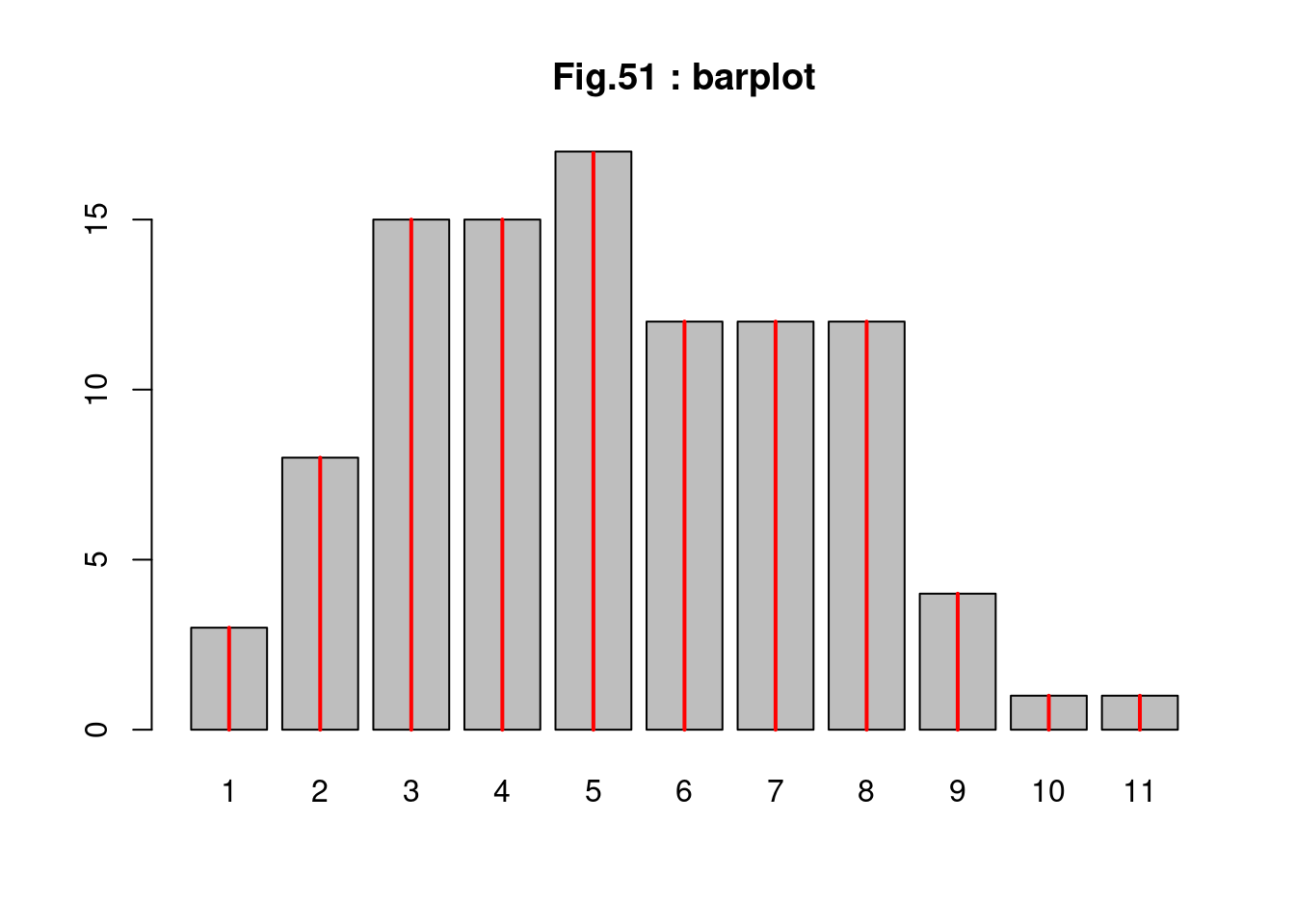
###### example of hist ##############################################
   str(islands)  # オブジェクト islands の属性等の表示
## Named num [1:48] 11506 5500 16988 2968 16 ...
## - attr(*, "names")= chr [1:48] "Africa" "Antarctica" "Asia" "Australia" ... islands # オブジェクト islands の表示## Africa Antarctica Asia Australia
## 11506 5500 16988 2968
## Axel Heiberg Baffin Banks Borneo
## 16 184 23 280
## Britain Celebes Celon Cuba
## 84 73 25 43
## Devon Ellesmere Europe Greenland
## 21 82 3745 840
## Hainan Hispaniola Hokkaido Honshu
## 13 30 30 89
## Iceland Ireland Java Kyushu
## 40 33 49 14
## Luzon Madagascar Melville Mindanao
## 42 227 16 36
## Moluccas New Britain New Guinea New Zealand (N)
## 29 15 306 44
## New Zealand (S) Newfoundland North America Novaya Zemlya
## 58 43 9390 32
## Prince of Wales Sakhalin South America Southampton
## 13 29 6795 16
## Spitsbergen Sumatra Taiwan Tasmania
## 15 183 14 26
## Tierra del Fuego Timor Vancouver Victoria
## 19 13 12 82 op <- par(mfrow = c(1, 2), cex.main=1.5)
(hist(islands)) # ヒストグラム(度数分布表)の表示と描画(左図)## $breaks
## [1] 0 2000 4000 6000 8000 10000 12000 14000 16000 18000
##
## $counts
## [1] 41 2 1 1 1 1 0 0 1
##
## $density
## [1] 4.270833e-04 2.083333e-05 1.041667e-05 1.041667e-05 1.041667e-05
## [6] 1.041667e-05 0.000000e+00 0.000000e+00 1.041667e-05
##
## $mids
## [1] 1000 3000 5000 7000 9000 11000 13000 15000 17000
##
## $xname
## [1] "islands"
##
## $equidist
## [1] TRUE
##
## attr(,"class")
## [1] "histogram" utils::str(hist(islands, col = "gray", labels = TRUE)) # 右図 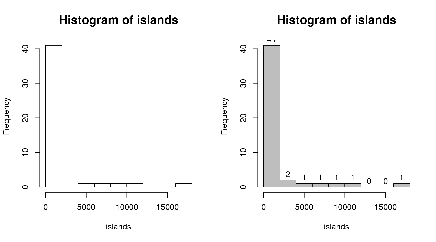
## List of 6
##  $ breaks  : num [1:10] 0 2000 4000 6000 8000 10000 12000 14000 16000 18000
##  $ counts  : int [1:9] 41 2 1 1 1 1 0 0 1
##  $ density : num [1:9] 4.27e-04 2.08e-05 1.04e-05 1.04e-05 1.04e-05 ...
##  $ mids    : num [1:9] 1000 3000 5000 7000 9000 11000 13000 15000 17000
##  $ xname   : chr "islands"
##  $ equidist: logi TRUE
##  - attr(*, "class")= chr "histogram"
# データの平方根変換と階級数を指定したヒストグラム(左図)
hist(sqrt(islands), br = 12, col = "lightblue", border = "pink")
# データの平方根変換と階級境界値を指定したヒストグラム(右図)
r <- hist(sqrt(islands),
br = c(4 * 0:5, 10 * 3:5, 70, 100, 140), col = "blue1")
# 度数を追加表示
text(r$mids, r$density, r$counts, adj = c(0.5, -0.5), col = "blue3")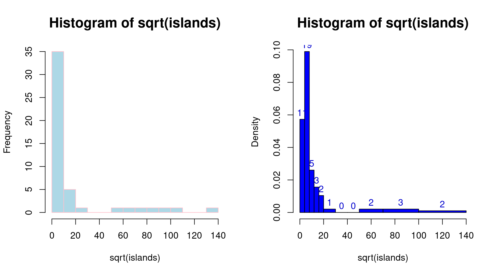
barplot
str(VADeaths)## num [1:5, 1:4] 11.7 18.1 26.9 41 66 8.7 11.7 20.3 30.9 54.3 ...
## - attr(*, "dimnames")=List of 2
## ..$ : chr [1:5] "50-54" "55-59" "60-64" "65-69" ...
## ..$ : chr [1:4] "Rural Male" "Rural Female" "Urban Male" "Urban Female" VADeaths## Rural Male Rural Female Urban Male Urban Female
## 50-54 11.7 8.7 15.4 8.4
## 55-59 18.1 11.7 24.3 13.6
## 60-64 26.9 20.3 37.0 19.3
## 65-69 41.0 30.9 54.6 35.1
## 70-74 66.0 54.3 71.1 50.0 barplot(VADeaths, plot = FALSE)## [1] 0.7 1.9 3.1 4.3 barplot(VADeaths, plot = FALSE, beside = TRUE)## [,1] [,2] [,3] [,4]
## [1,] 1.5 7.5 13.5 19.5
## [2,] 2.5 8.5 14.5 20.5
## [3,] 3.5 9.5 15.5 21.5
## [4,] 4.5 10.5 16.5 22.5
## [5,] 5.5 11.5 17.5 23.5 mp <- barplot(VADeaths, main="Fig.53 : : Death Rates in Virginia (VADeaths)")
tot <- colMeans(VADeaths) # 列毎の平均
text(mp, tot + 3, format(tot), xpd = TRUE, col = "blue") # 列平均の追記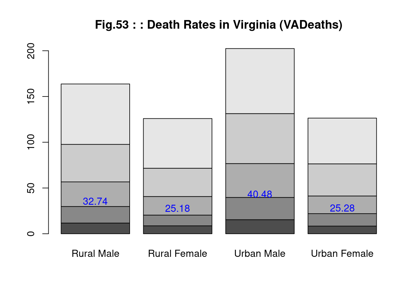
  if(1){
    barplot(VADeaths, beside = TRUE,
            col = c("lightblue", "mistyrose", "lightcyan", "lavender",
                    "cornsilk"),
            legend = rownames(VADeaths), ylim = c(0, 100))

    title(main = "Fig.54 : Death Rates in Virginia", font.main = 4)
    } # end of if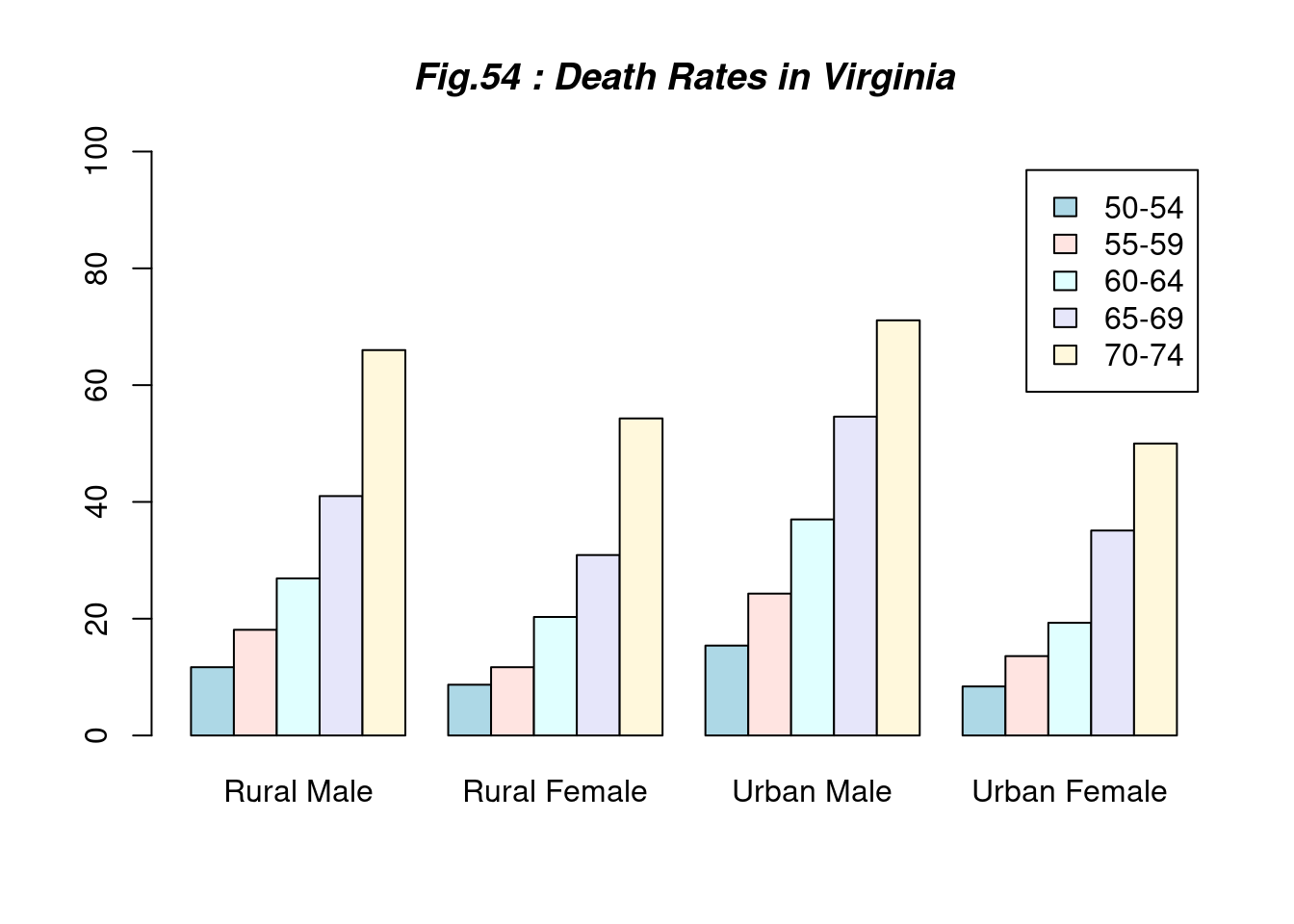
    hh <- t(VADeaths)[, 5:1]
    mybarcol <- "gray20"
    mp <- barplot(hh, beside = TRUE,
                  col = c("lightblue", "mistyrose", "lightcyan","lavender"),
                  legend = colnames(VADeaths),
                  ylim = c(0, 100),
                  main = "Fig.55 : Death Rates in Virginia", font.main = 4,
                  sub = "Faked upper 2*sigma error bars")
    segments(mp, hh, mp, hh + 2 * sqrt(1000 * hh/100),
              col = mybarcol, lwd = 1.5)
    stopifnot(dim(mp) == dim(hh))
    mtext(side = 1, at = colMeans(mp), line = -2,
          text = paste("Mean", formatC(colMeans(hh))), col = "red")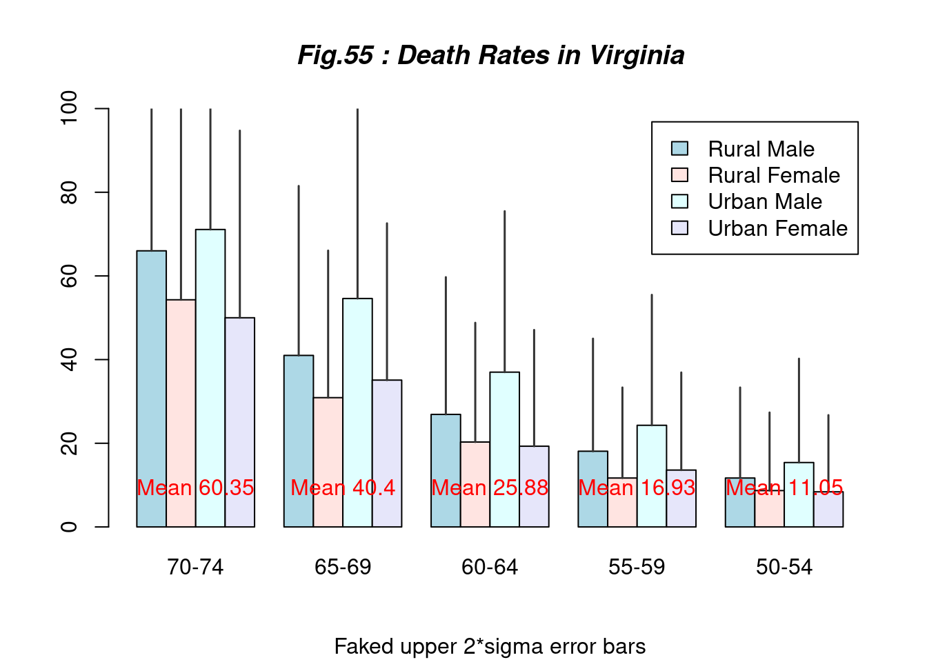
領域の塗りつぶし
polygon
    plot(dnorm,-4,4)              # N(0,1)のpdfを区間[-4,4]で描画する
    n <- 3
    xvals <- seq(-2,2,length=n)   # 領域をx軸方向にn個の多角形(台形)に等分割
    dvals <- dnorm(xvals)         # 対応するグラフの高さ(関数値)を求める
    xvals
## [1] -2 0 2 dvals## [1] 0.05399097 0.39894228 0.05399097 c(xvals,rev(xvals))## [1] -2 0 2 2 0 -2 c(rep(0,n),rev(dvals))## [1] 0.00000000 0.00000000 0.00000000 0.05399097 0.39894228 0.05399097 polygon(c(xvals,rev(xvals)),c(rep(0,n),rev(dvals)),col="gray")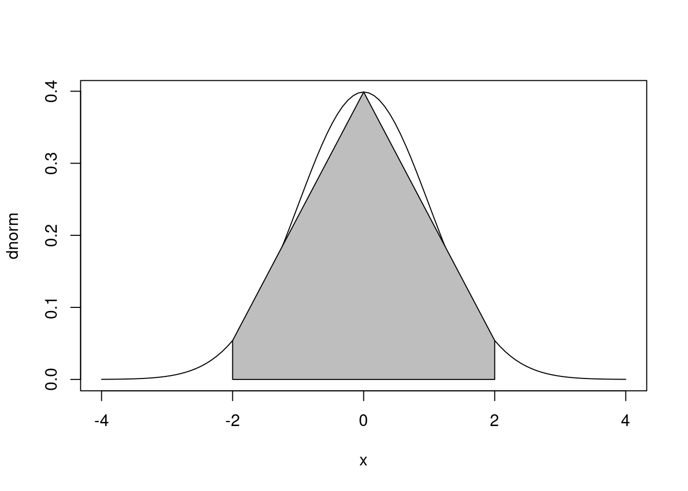
    # xvals,rep(0,n) の組合せでx軸上の辺を結ぶ
    # rev(xvals),rev(dvals) の組合せでグラフに沿った辺を結ぶ
polygon と確率
f20 <- function(x){0*x}         # 関数f2を準備する
f20(3)
## [1] 0# 描画関数 polyf を作成する
polyf <- function(xl, xr, f1, f2, x0, x1, n=50, col="gray", debug=FALSE, ...){
if (debug) {
txt <- paste(" ** polyf ** \n",
" 区間 [xl, xr] 上に関数 f1(x), f2(x) を描画し, 区間 [x0, x1] 上で ",
" f1(x), f2(x) で囲まれた領域を表示する\n", sep="")
cat(txt) }
plot(f1, xl, xr, ...) # 関数f1(x) (関数名で指定)を区間[xl, xr]で描画する
curve(f2, xl, xr, add=TRUE) # 関数f2(x) (関数名で指定)を区間[xl, xr]で追加描画する
xv <- seq(x0, x1, length=n) # 区間[x0,x1]をn分割した点ベクトル
yv1 <- f1(xv) # 分割点での関数f1の関数値ベクトル
yv2 <- f2(xv) # 分割点での関数f2の関数値ベクトル
xp <- c(xv, rev(xv)) # 一筆書きx0...x1...x0に対応するベクトル
yp <- c(yv1, rev(yv2)) # xpに対応する関数値ベクトル
if (debug > 1) {
cat("xp =",xp,"\n"); cat("yp ~",yp,"\n")
}
polygon(xp,yp,col=col, ...) # 関数polygon()を適用
} # end of polyf
polyf(-4, 4, dnorm, f20, 2, 10, main="Normal Dist.", ylab="f(x)", debug=TRUE)## ** polyf **
## 区間 [xl, xr] 上に関数 f1(x), f2(x) を描画し, 区間 [x0, x1] 上で f1(x), f2(x) で囲まれた領域を表示する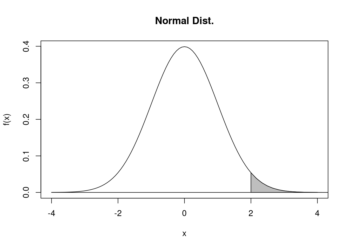 \[ 上側確率~~ Q(2) = P\{ X > 2\} = 0.0227501\]
par(mfrow=c(1,2))
polyf(-pi/2, 3/2*pi, sin, cos, 0, pi, ylab="f(x)")
polyf(-pi/2, 3/2*pi, sin, f20, 0, pi, ylab="f(x)", debug=T)
## ** polyf **
## 区間 [xl, xr] 上に関数 f1(x), f2(x) を描画し, 区間 [x0, x1] 上で f1(x), f2(x) で囲まれた領域を表示する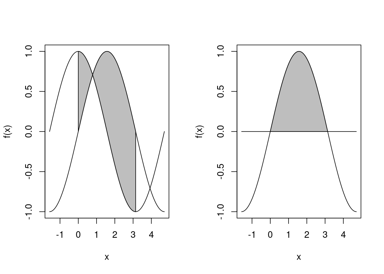
関数 par() の設定例
     op <- par(mfrow = c(2, 2), # 2 x 2 pictures on one plot
               pty = "s")       # square plotting region,
                                # independent of device size

     ## At end of plotting, reset to previous settings:
     par(op)

     ## Alternatively,
     op <- par(no.readonly = TRUE) # the whole list of settable par's.
     ## do lots of plotting and par(.) calls, then reset:
     par(op)
     ## Note this is not in general good practice

     par("ylog") # FALSE
## [1] FALSE plot(1 : 12, log = "y")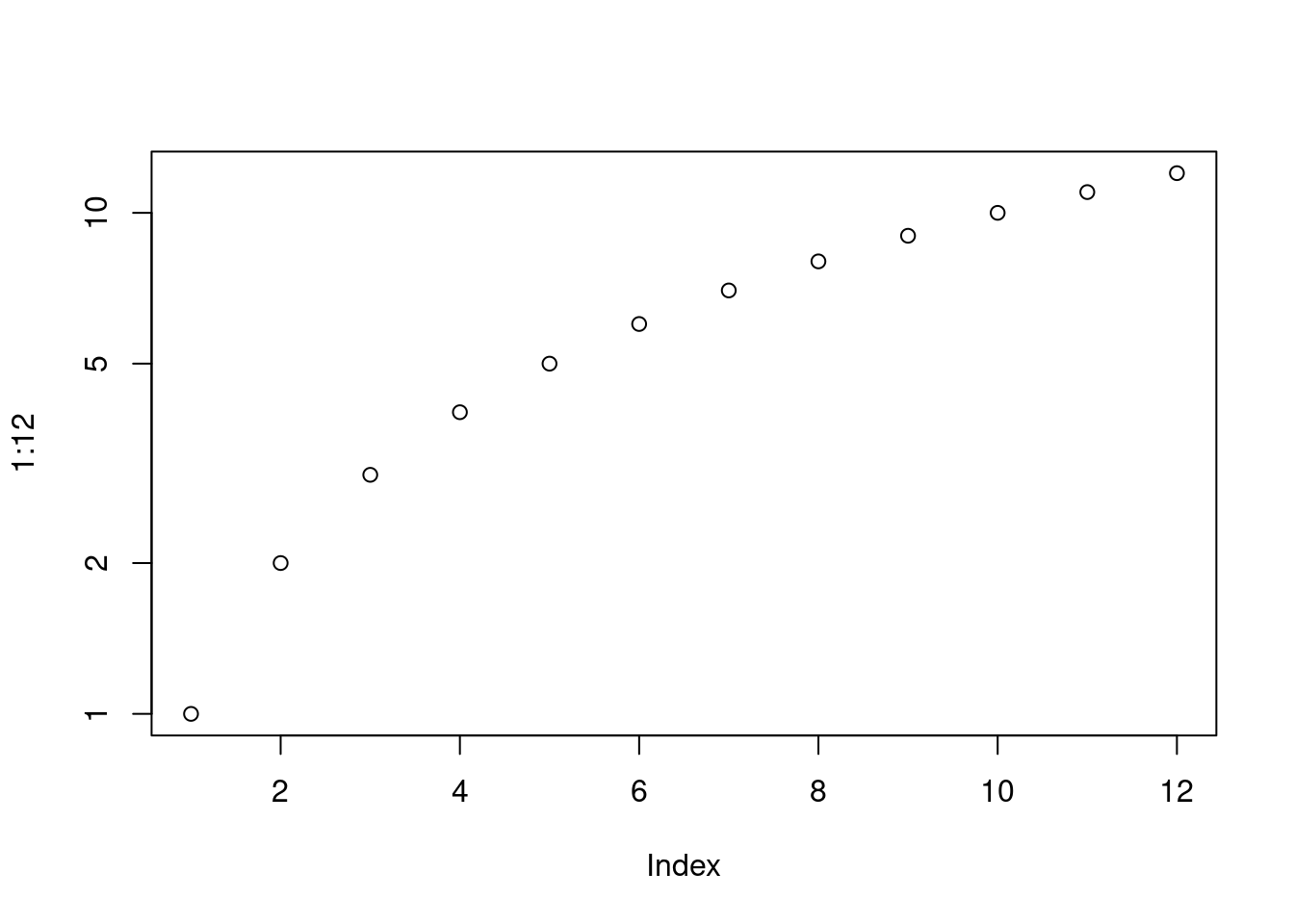
par("ylog") # TRUE## [1] TRUE plot(1:2, xaxs = "i") # 'inner axis' w/o extra space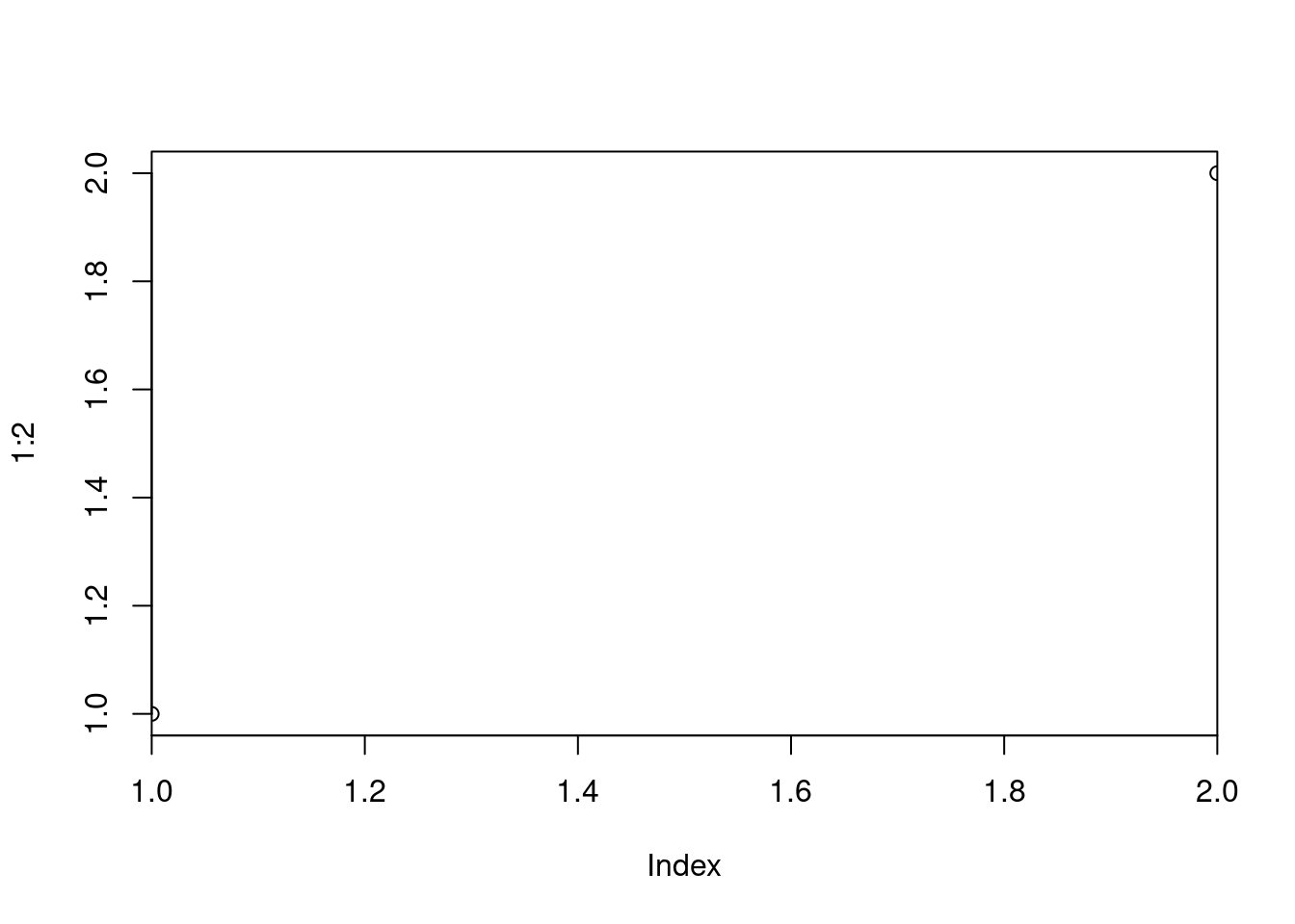
par(c("usr", "xaxp"))## $usr
## [1] 1.00 2.00 0.96 2.04
##
## $xaxp
## [1] 1 2 5 ( nr.prof <-
c(prof.pilots = 16, lawyers = 11, farmers = 10, salesmen = 9, physicians = 9,
mechanics = 6, policemen = 6, managers = 6, engineers = 5, teachers = 4,
housewives = 3, students = 3, armed.forces = 1))## prof.pilots lawyers farmers salesmen physicians mechanics
## 16 11 10 9 9 6
## policemen managers engineers teachers housewives students
## 6 6 5 4 3 3
## armed.forces
## 1 par(las = 3)
barplot(rbind(nr.prof)) # R 0.63.2: shows alignment problem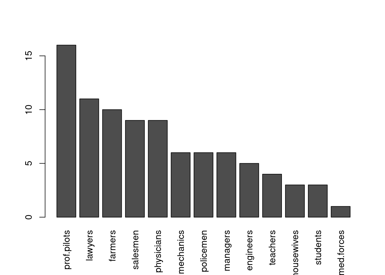
     par(las = 0)  # reset to default

     require(grDevices) # for gray
     ## 'fg' use:
     plot(1:12, type = "b", main = "'fg' : axes, ticks and box in gray",
          fg = gray(0.7), bty = "7" , sub = R.version.string)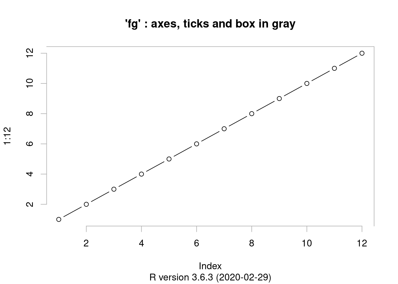
     ex <- function() {
        old.par <- par(no.readonly = TRUE) # all par settings which
                                           # could be changed.
        on.exit(par(old.par))
        ## ...
        ## ... do lots of par() settings and plots
        ## ...
        invisible() #-- now,  par(old.par)  will be executed
     }
     ex()

     ## Line types
     showLty <- function(ltys, xoff = 0, ...) {
        stopifnot((n <- length(ltys)) >= 1)
        op <- par(mar = rep(.5,4)); on.exit(par(op))
        plot(0:1, 0:1, type = "n", axes = FALSE, ann = FALSE)
        y <- (n:1)/(n+1)
        clty <- as.character(ltys)
        mytext <- function(x, y, txt)
           text(x, y, txt, adj = c(0, -.3), cex = 0.8, ...)
        abline(h = y, lty = ltys, ...); mytext(xoff, y, clty)
        y <- y - 1/(3*(n+1))
        abline(h = y, lty = ltys, lwd = 2, ...)
        mytext(1/8+xoff, y, paste(clty," lwd = 2"))
     }
     showLty(c("solid", "dashed", "dotted", "dotdash", "longdash", "twodash"))
     par(new = TRUE)  # the same:
     showLty(c("solid", "44", "13", "1343", "73", "2262"), xoff = .2, col = 2)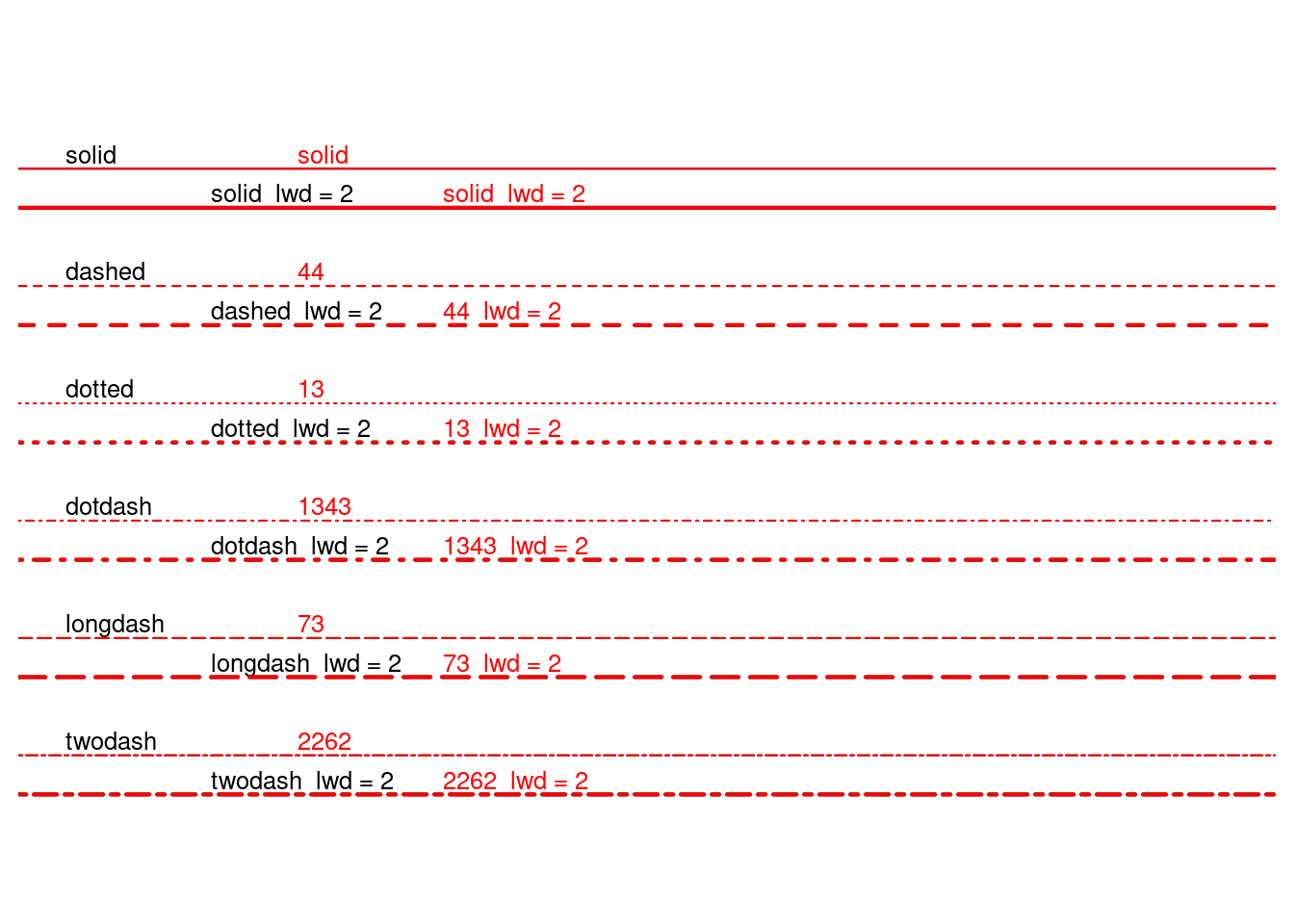
showLty(c("11", "22", "33", "44", "12", "13", "14", "21", "31"))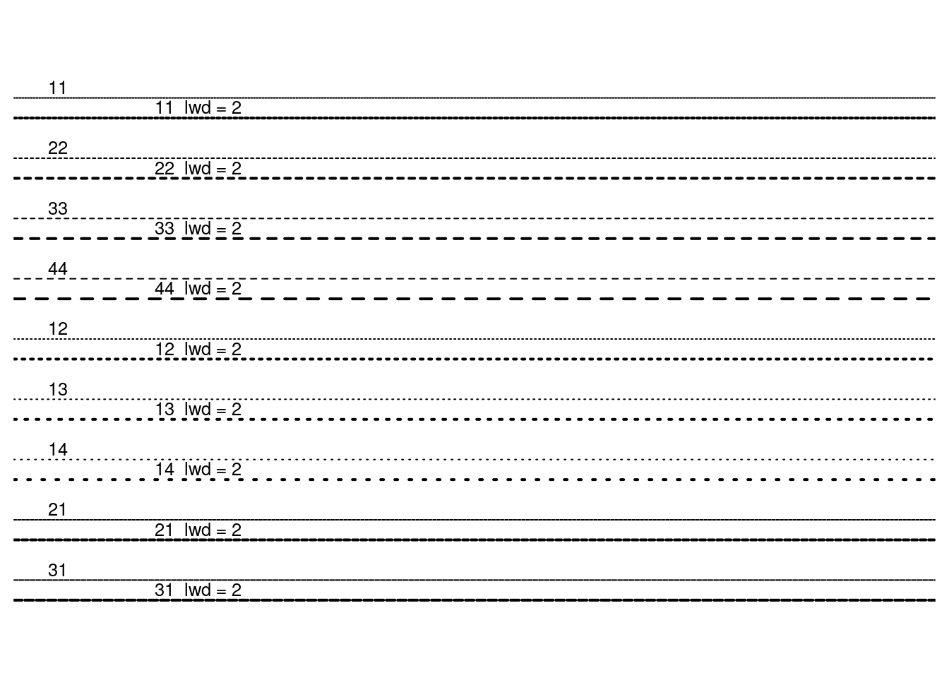
パッケージ lowess の作図
lowess                  package:stats                  R Documentation

Scatter Plot Smoothing

Description:

     This function performs the computations for the _LOWESS_ smoother
     which uses locally-weighted polynomial regression (see the
     references).

Usage:

     lowess(x, y = NULL, f = 2/3, iter = 3, delta = 0.01 * diff(range(x)))

Arguments:

    x, y: vectors giving the coordinates of the points in the scatter
          plot.  Alternatively a single plotting structure can be
          specified - see ‘xy.coords’.

       f: the smoother span. This gives the proportion of points in the
          plot which influence the smooth at each value.  Larger values
          give more smoothness.

    iter: the number of ‘robustifying’ iterations which should be
          performed.  Using smaller values of ‘iter’ will make
          ‘lowess’ run faster.

delta: See ‘Details’. Defaults to 1/100th of the range of ‘x’. str(cars)## 'data.frame': 50 obs. of 2 variables:
## $ speed: num 4 4 7 7 8 9 10 10 10 11 ...
## $ dist : num 2 10 4 22 16 10 18 26 34 17 ... str(lowess(cars))## List of 2
## $ x: num [1:50] 4 4 7 7 8 9 10 10 10 11 ...
## $ y: num [1:50] 4.97 4.97 13.12 13.12 15.86 ... plot(cars, main = "lowess(cars)")
lines(lowess(cars), col = 2)
lines(lowess(cars, f = .2), col = 3)
legend(5, 120, c(paste("f = ", c("2/3", ".2"))), lty = 1, col = 2:3)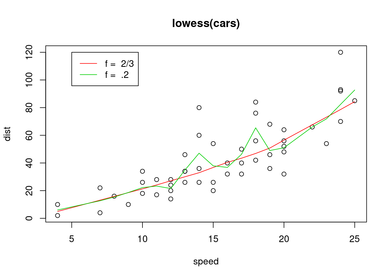
補足
hp <- help(par)
hp
op <- par()
str(op)
## List of 72
## $ xlog : logi FALSE
## $ ylog : logi FALSE
## $ adj : num 0.5
## $ ann : logi TRUE
## $ ask : logi FALSE
## $ bg : chr "white"
## $ bty : chr "o"
## $ cex : num 1
## $ cex.axis : num 1
## $ cex.lab : num 1
## $ cex.main : num 1.2
## $ cex.sub : num 1
## $ cin : num [1:2] 0.15 0.2
## $ col : chr "black"
## $ col.axis : chr "black"
## $ col.lab : chr "black"
## $ col.main : chr "black"
## $ col.sub : chr "black"
## $ cra : num [1:2] 28.8 38.4
## $ crt : num 0
## $ csi : num 0.2
## $ cxy : num [1:2] 0.026 0.0633
## $ din : num [1:2] 7 5
## $ err : int 0
## $ family : chr ""
## $ fg : chr "black"
## $ fig : num [1:4] 0 1 0 1
## $ fin : num [1:2] 7 5
## $ font : int 1
## $ font.axis: int 1
## $ font.lab : int 1
## $ font.main: int 2
## $ font.sub : int 1
## $ lab : int [1:3] 5 5 7
## $ las : int 0
## $ lend : chr "round"
## $ lheight : num 1
## $ ljoin : chr "round"
## $ lmitre : num 10
## $ lty : chr "solid"
## $ lwd : num 1
## $ mai : num [1:4] 1.02 0.82 0.82 0.42
## $ mar : num [1:4] 5.1 4.1 4.1 2.1
## $ mex : num 1
## $ mfcol : int [1:2] 1 1
## $ mfg : int [1:4] 1 1 1 1
## $ mfrow : int [1:2] 1 1
## $ mgp : num [1:3] 3 1 0
## $ mkh : num 0.001
## $ new : logi FALSE
## $ oma : num [1:4] 0 0 0 0
## $ omd : num [1:4] 0 1 0 1
## $ omi : num [1:4] 0 0 0 0
## $ page : logi TRUE
## $ pch : int 1
## $ pin : num [1:2] 5.76 3.16
## $ plt : num [1:4] 0.117 0.94 0.204 0.836
## $ ps : int 12
## $ pty : chr "m"
## $ smo : num 1
## $ srt : num 0
## $ tck : num NA
## $ tcl : num -0.5
## $ usr : num [1:4] 0 1 0 1
## $ xaxp : num [1:3] 0 1 5
## $ xaxs : chr "r"
## $ xaxt : chr "s"
## $ xpd : logi FALSE
## $ yaxp : num [1:3] 0 1 5
## $ yaxs : chr "r"
## $ yaxt : chr "s"
## $ ylbias : num 0.2quartzFonts()## $serif
## [1] "Times-Roman" "Times-Bold" "Times-Italic" "Times-BoldItalic"
##
## $sans
## [1] "Helvetica" "Helvetica-Bold" "Helvetica-Oblique"
## [4] "Helvetica-BoldOblique"
##
## $mono
## [1] "Courier" "Courier-Bold" "Courier-Oblique"
## [4] "Courier-BoldOblique"