w2018.Rmd Memo

逆行列
- ヒルベルト(部分)行列の特異値分解
固有値分解
特異値分解
乱数
円の最小2乗法
球の最小2乗法
R言語私用ライブラリRLIBのメモ: ex-persp.Rnw
End

逆行列

hilbert <- function(n) { i <- 1:n; 1 / outer(i - 1, i, "+") }   # ヒルベルト行列
h5 <- hilbert(5); h5    # 5x5 のヒルベルト行列 h5 を作成

##           [,1]      [,2]      [,3]      [,4]      [,5]
## [1,] 1.0000000 0.5000000 0.3333333 0.2500000 0.2000000
## [2,] 0.5000000 0.3333333 0.2500000 0.2000000 0.1666667
## [3,] 0.3333333 0.2500000 0.2000000 0.1666667 0.1428571
## [4,] 0.2500000 0.2000000 0.1666667 0.1428571 0.1250000
## [5,] 0.2000000 0.1666667 0.1428571 0.1250000 0.1111111

sh5 <- solve(h5); sh5   # h5 の逆行列 sh5 を求める

##       [,1]   [,2]    [,3]    [,4]   [,5]
## [1,]    25   -300    1050   -1400    630
## [2,]  -300   4800  -18900   26880 -12600
## [3,]  1050 -18900   79380 -117600  56700
## [4,] -1400  26880 -117600  179200 -88200
## [5,]   630 -12600   56700  -88200  44100

round(sh5 %*% h5, 7)    # 有効桁数を7とした表示

##      [,1] [,2] [,3] [,4] [,5]
## [1,]    1    0    0    0    0
## [2,]    0    1    0    0    0
## [3,]    0    0    1    0    0
## [4,]    0    0    0    1    0
## [5,]    0    0    0    0    1

svd(h5)$d

## [1] 1.567051e+00 2.085342e-01 1.140749e-02 3.058980e-04 3.287929e-06

eigen(h5)$values        #

## [1] 1.567051e+00 2.085342e-01 1.140749e-02 3.058980e-04 3.287929e-06

eigen(hilbert(15))$values

##  [1]  1.845928e+00  4.266280e-01  5.721209e-02  5.639835e-03  4.364766e-04
##  [6]  2.710854e-05  1.361582e-06  5.528988e-08  1.802960e-09  4.657786e-11
## [11]  9.321636e-13  1.394583e-14  1.459475e-16  1.152248e-17 -5.798811e-18

out <- try(solve(hilbert(15)),TRUE)
print(out)

## [1] "Error in solve.default(hilbert(15)) : \n  system is computationally singular: reciprocal condition number = 1.5434e-18\n"
## attr(,"class")
## [1] "try-error"
## attr(,"condition")
## <simpleError in solve.default(hilbert(15)): system is computationally singular: reciprocal condition number = 1.5434e-18>

ヒルベルト(部分)行列の特異値分解

     hilbert <- function(n) { i <- 1:n; 1 / outer(i - 1, i, "+") }  # ヒルベルト行列
     X <- hilbert(9)[, 1:6]  # 9x6 行列 X を作成
     (s <- svd(X))

## $d
## [1] 1.668433e+00 2.773727e-01 2.223722e-02 1.084693e-03 3.243788e-05
## [6] 5.234864e-07
## 
## $u
##             [,1]       [,2]        [,3]        [,4]        [,5]        [,6]
##  [1,] -0.7244999  0.6265620  0.27350003 -0.08526902  0.02074121 -0.00402455
##  [2,] -0.4281556 -0.1298781 -0.64293597  0.55047428 -0.27253421  0.09281592
##  [3,] -0.3121985 -0.2803679 -0.33633240 -0.31418014  0.61632113 -0.44090375
##  [4,] -0.2478932 -0.3141885 -0.06931246 -0.44667149  0.02945426  0.53011986
##  [5,] -0.2063780 -0.3140734  0.10786005 -0.30241655 -0.35566839  0.23703838
##  [6,] -0.1771408 -0.3026808  0.22105904 -0.09041508 -0.38878613 -0.26044927
##  [7,] -0.1553452 -0.2877310  0.29280775  0.11551327 -0.19285565 -0.42094482
##  [8,] -0.1384280 -0.2721599  0.33783778  0.29312535  0.11633231 -0.16079025
##  [9,] -0.1248940 -0.2571250  0.36542543  0.43884649  0.46496714  0.43459954
## 
## $v
##            [,1]       [,2]       [,3]        [,4]        [,5]         [,6]
## [1,] -0.7364928  0.6225002  0.2550021 -0.06976287  0.01328234 -0.001588146
## [2,] -0.4432826 -0.1818705 -0.6866860  0.50860089 -0.19626669  0.041116974
## [3,] -0.3274789 -0.3508553 -0.2611139 -0.50473697  0.61605641 -0.259215626
## [4,] -0.2626469 -0.3921783  0.1043599 -0.43747940 -0.40833605  0.638901622
## [5,] -0.2204199 -0.3945644  0.3509658  0.01612426 -0.46427916 -0.675826789
## [6,] -0.1904420 -0.3831871  0.5110654  0.53856351  0.44663632  0.257248908

     D <- diag(s$d)
     s$u %*% D %*% t(s$v) #  X = U D V'

##            [,1]      [,2]       [,3]       [,4]       [,5]       [,6]
##  [1,] 1.0000000 0.5000000 0.33333333 0.25000000 0.20000000 0.16666667
##  [2,] 0.5000000 0.3333333 0.25000000 0.20000000 0.16666667 0.14285714
##  [3,] 0.3333333 0.2500000 0.20000000 0.16666667 0.14285714 0.12500000
##  [4,] 0.2500000 0.2000000 0.16666667 0.14285714 0.12500000 0.11111111
##  [5,] 0.2000000 0.1666667 0.14285714 0.12500000 0.11111111 0.10000000
##  [6,] 0.1666667 0.1428571 0.12500000 0.11111111 0.10000000 0.09090909
##  [7,] 0.1428571 0.1250000 0.11111111 0.10000000 0.09090909 0.08333333
##  [8,] 0.1250000 0.1111111 0.10000000 0.09090909 0.08333333 0.07692308
##  [9,] 0.1111111 0.1000000 0.09090909 0.08333333 0.07692308 0.07142857

     t(s$u) %*% X %*% s$v #  D = U' X V

##               [,1]          [,2]          [,3]          [,4]          [,5]
## [1,]  1.668433e+00  4.163336e-17  1.665335e-16 -2.775558e-16  8.326673e-17
## [2,]  1.214306e-16  2.773727e-01  0.000000e+00  2.775558e-17  2.775558e-17
## [3,]  7.762888e-17 -4.336809e-17  2.223722e-02  1.734723e-17 -1.301043e-17
## [4,] -7.956689e-17  3.699840e-17 -6.722053e-18  1.084693e-03 -2.981556e-18
## [5,]  3.843116e-17  3.057111e-17  1.626727e-17  3.926845e-18  3.243788e-05
## [6,]  3.097149e-17  5.394012e-19 -1.123645e-17 -6.214403e-18  1.613745e-17
##               [,6]
## [1,] -9.714451e-17
## [2,]  3.469447e-17
## [3,]  1.170938e-17
## [4,] -1.910906e-17
## [5,] -2.688483e-18
## [6,]  5.234864e-07

固有値分解

### 1. 実非対称行列の固有値分解;
A <- matrix(c(1, 0.5, 0.25, 0.75), ncol=2, byrow=T); A;

##      [,1] [,2]
## [1,] 1.00 0.50
## [2,] 0.25 0.75

ans <- eigen(A); ans;

## eigen() decomposition
## $values
## [1] 1.25 0.50
## 
## $vectors
##           [,1]       [,2]
## [1,] 0.8944272 -0.7071068
## [2,] 0.4472136  0.7071068

G <- ans$vectors; G;

##           [,1]       [,2]
## [1,] 0.8944272 -0.7071068
## [2,] 0.4472136  0.7071068

D <- diag(ans$values); D;

##      [,1] [,2]
## [1,] 1.25  0.0
## [2,] 0.00  0.5

B <- G %*% D %*% solve(G)
B;

##      [,1] [,2]
## [1,] 1.00 0.50
## [2,] 0.25 0.75

### 2. 実対称行列の固有値分解;
A <- matrix(c(1, 0.5, 0.5, 1), ncol=2, byrow=T); A;

##      [,1] [,2]
## [1,]  1.0  0.5
## [2,]  0.5  1.0

ans <- eigen(A); ans;

## eigen() decomposition
## $values
## [1] 1.5 0.5
## 
## $vectors
##           [,1]       [,2]
## [1,] 0.7071068 -0.7071068
## [2,] 0.7071068  0.7071068

G <- ans$vectors; G;

##           [,1]       [,2]
## [1,] 0.7071068 -0.7071068
## [2,] 0.7071068  0.7071068

D <- diag(ans$values); D;

##      [,1] [,2]
## [1,]  1.5  0.0
## [2,]  0.0  0.5

B <- G %*% D %*% solve(G)
B;

##      [,1] [,2]
## [1,]  1.0  0.5
## [2,]  0.5  1.0

### 3. 実対称行列(ランク落ち)の固有値分解;
A <- matrix(c(1, 1, 1, 1), ncol=2, byrow=T); A;

##      [,1] [,2]
## [1,]    1    1
## [2,]    1    1

ans <- eigen(A); ans;

## eigen() decomposition
## $values
## [1] 2 0
## 
## $vectors
##           [,1]       [,2]
## [1,] 0.7071068 -0.7071068
## [2,] 0.7071068  0.7071068

G <- ans$vectors; G;

##           [,1]       [,2]
## [1,] 0.7071068 -0.7071068
## [2,] 0.7071068  0.7071068

D <- diag(ans$values); D;

##      [,1] [,2]
## [1,]    2    0
## [2,]    0    0

B <- G %*% D %*% solve(G)
B;

##      [,1] [,2]
## [1,]    1    1
## [2,]    1    1

### 4. 実対称行列(自明)の固有値分解;
A <- matrix(c(2, 0, 0, 2), ncol=2, byrow=T); A;

##      [,1] [,2]
## [1,]    2    0
## [2,]    0    2

ans <- eigen(A); ans;

## eigen() decomposition
## $values
## [1] 2 2
## 
## $vectors
##      [,1] [,2]
## [1,]    0   -1
## [2,]    1    0

G <- ans$vectors; G;

##      [,1] [,2]
## [1,]    0   -1
## [2,]    1    0

D <- diag(ans$values); D;

##      [,1] [,2]
## [1,]    2    0
## [2,]    0    2

B <- G %*% D %*% solve(G)
B;

##      [,1] [,2]
## [1,]    2    0
## [2,]    0    2

特異値分解

### 1. 実行列の特異値分解 A = U D V' ;
p <- 3;
A <- matrix(c(1, 1, 0,   
              1, 1, 0,  
              1, 0, 1,  
              1, 0, 1), ncol=p, byrow=T); A;

##      [,1] [,2] [,3]
## [1,]    1    1    0
## [2,]    1    1    0
## [3,]    1    0    1
## [4,]    1    0    1

ans <- svd(A); ans;

## $d
## [1] 2.449490e+00 1.414214e+00 8.546501e-17
## 
## $u
##      [,1] [,2]          [,3]
## [1,] -0.5 -0.5  7.071068e-01
## [2,] -0.5 -0.5 -7.071068e-01
## [3,] -0.5  0.5  0.000000e+00
## [4,] -0.5  0.5  1.110223e-16
## 
## $v
##            [,1]          [,2]       [,3]
## [1,] -0.8164966 -1.541976e-16  0.5773503
## [2,] -0.4082483 -7.071068e-01 -0.5773503
## [3,] -0.4082483  7.071068e-01 -0.5773503

ev <- ans$d;
for (i in p:1) {if (abs(ev[i]) < 1.0e-15) rnk <- i-1};
rnk;

## [1] 2

### rank まで再計算する；
ans <- svd(A,nu=rnk,nv=rnk); ans;

## $d
## [1] 2.449490e+00 1.414214e+00 8.546501e-17
## 
## $u
##      [,1] [,2]
## [1,] -0.5 -0.5
## [2,] -0.5 -0.5
## [3,] -0.5  0.5
## [4,] -0.5  0.5
## 
## $v
##            [,1]          [,2]
## [1,] -0.8164966 -1.541976e-16
## [2,] -0.4082483 -7.071068e-01
## [3,] -0.4082483  7.071068e-01

U <- ans$u; U;

##      [,1] [,2]
## [1,] -0.5 -0.5
## [2,] -0.5 -0.5
## [3,] -0.5  0.5
## [4,] -0.5  0.5

ans$d;

## [1] 2.449490e+00 1.414214e+00 8.546501e-17

ans$d[1:rnk];

## [1] 2.449490 1.414214

D <- diag(ans$d[1:rnk]); D;

##         [,1]     [,2]
## [1,] 2.44949 0.000000
## [2,] 0.00000 1.414214

V <- ans$v
B <- U %*% D %*% t(V)
B;

##      [,1]         [,2]          [,3]
## [1,]    1 1.000000e+00 -1.665335e-16
## [2,]    1 1.000000e+00 -1.665335e-16
## [3,]    1 5.551115e-17  1.000000e+00
## [4,]    1 5.551115e-17  1.000000e+00

### 2. A'A の固有値分解 A'A = V D^2 V' ;
ATA <- t(A) %*% A; ATA;

##      [,1] [,2] [,3]
## [1,]    4    2    2
## [2,]    2    2    0
## [3,]    2    0    2

eigen(ATA);

## eigen() decomposition
## $values
## [1] 6.000000e+00 2.000000e+00 3.552714e-15
## 
## $vectors
##           [,1]       [,2]       [,3]
## [1,] 0.8164966  0.0000000  0.5773503
## [2,] 0.4082483 -0.7071068 -0.5773503
## [3,] 0.4082483  0.7071068 -0.5773503

### 3. 射影行列 Q = U U';
Q <- U %*% t(U);  Q;

##      [,1] [,2] [,3] [,4]
## [1,]  0.5  0.5  0.0  0.0
## [2,]  0.5  0.5  0.0  0.0
## [3,]  0.0  0.0  0.5  0.5
## [4,]  0.0  0.0  0.5  0.5

乱数

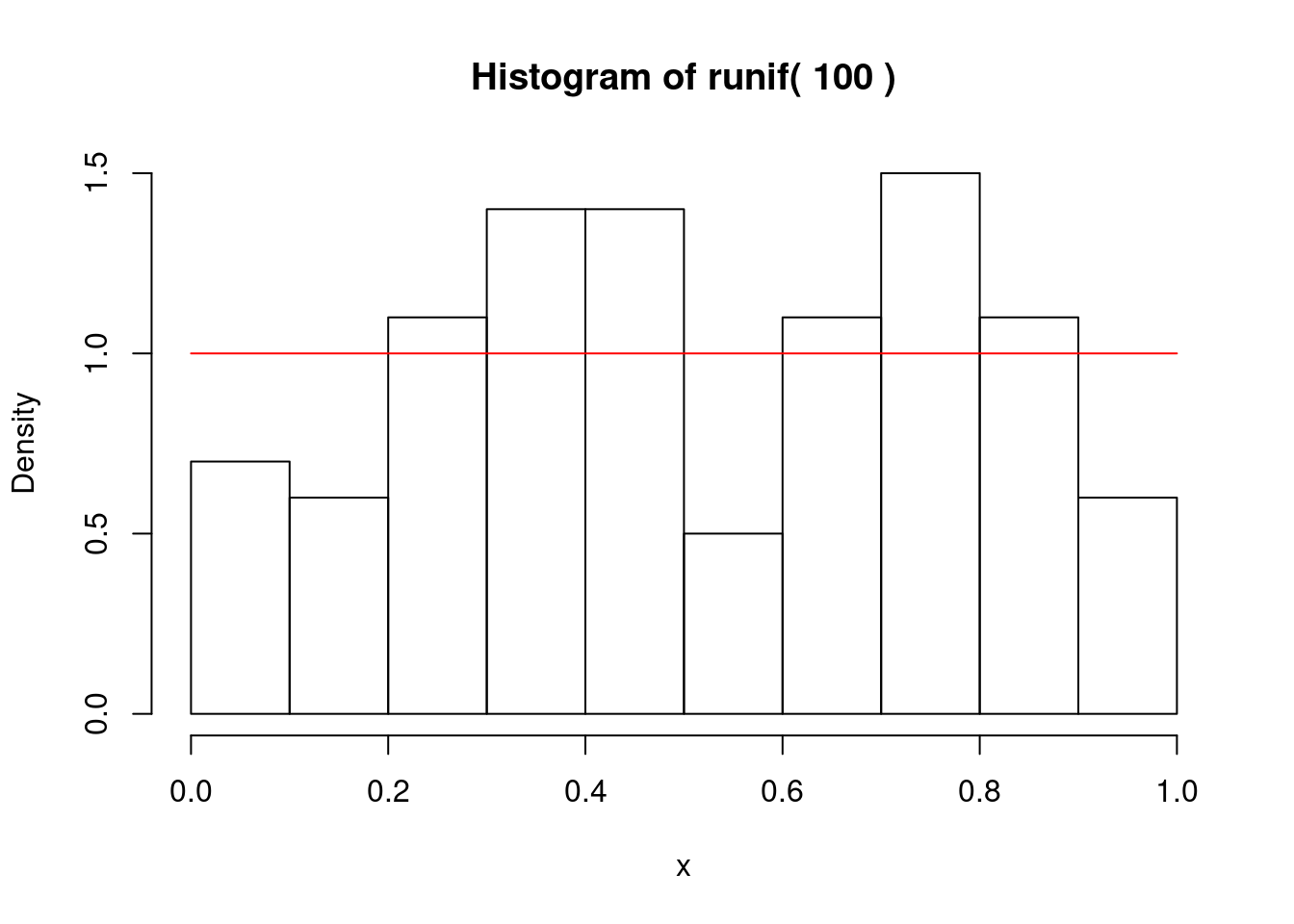
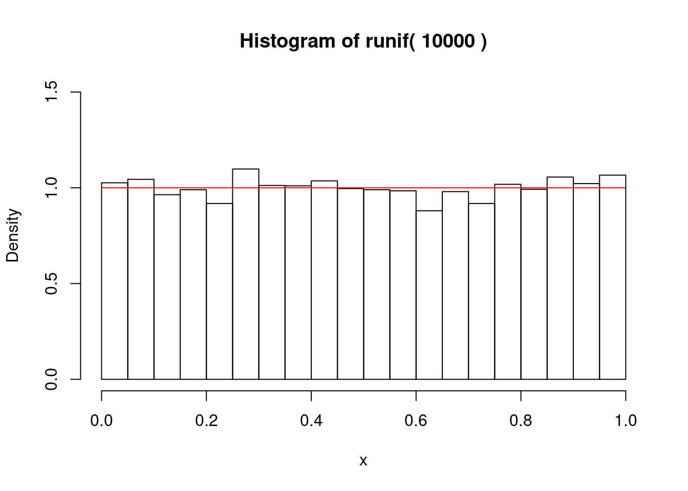
一様乱数

if (1) {
#  postscript("Rfig-1a.eps",height=18,horizontal=F)
#  par(mfrow=c(2,1),cex.main=1.5,cex.axis=1.5,lwd=1.5)
  nc <- c(100,10000)
  for (i in 1:length(nc)) {
    set.seed(1)
    n <- nc[i]
    x <- runif(n)
    gmain <- paste("Histogram of runif(",n,")")
    hist(x,freq=F,main=gmain,xlim=c(0,1),ylim=c(0,1.5))
    curve(dunif,0,1,add=T,col="red")
    } 
#  graphics.off()
  }

指数乱数

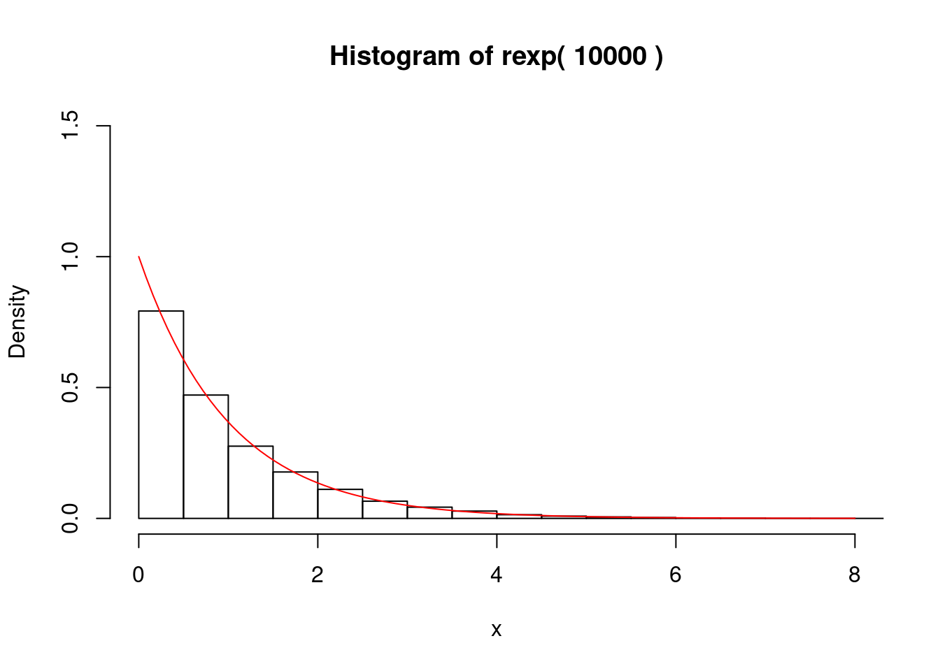
確率密度関数\(f(x)\)が\[ f(x) = \lambda\, e^{- \lambda x} \quad (x \ge 0) \] で表せる確率分布を「母数\(\lambda\)の指数分布」といい，\(X \sim {\rm Ex} (\lambda)\) と記す．このとき，分布関数\(F(x) = P\{ X < x\}\)は\(F(x) = 1 - e^{-\lambda x}\) で表せる．\(\lambda=1\)のときの指数分布の密度関数と分布関数を以下に示す．

###　指数分布の密度関数と分布関数のグラフ
# postscript("Rfig-2a.eps",horizontal=F)
par(mfrow=c(1,2),cex=1.2,lwd=1.5)
f <- function(x){dexp(x,rate=1.0)} # 確率密度関数
curve(f,0,8,col="red",main="Density Func")
F <- function(x){pexp(x,rate=1.0)} # 分布関数
curve(F,0,8,col="red",main="Cumulative Density Func")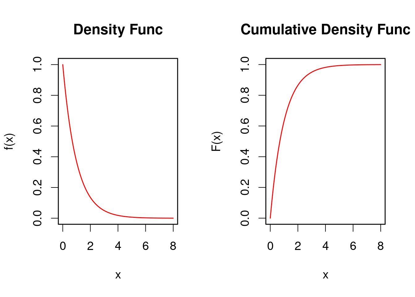

#graphics.off()
rm(f,F)

分布関数のグラフ(右図)より，\(y=F(x)=1 - e^{- x}\)を\(x\)について解くと，\(x = - \log(1-y)\) を得る．よって，\(y\)を一様乱数とすると，\(x = - \log(1-y)\)で定まる\(x\)は指数分布に従う確率変数の実現値，すなわち，指数乱数を得る．これを逆関数法による乱数変換という．以下にRによる実行例を示す．

### 指数乱数 F(x) = 1 - e^(-x) = y : -x = log(1-y)
if (1) {
#  postscript("Rfig-2.eps",height=6,horizontal=F); 
#    par(mfrow=c(1,1),cex.main=1.5,cex.axis=1.5,lwd=1.5)
    set.seed(1)
    n <- 10000
    y <- runif(n)
    x <- -log(1-y)
    gmain <- paste("Histogram of rexp(",n,")")
    hist(x,freq=F,main=gmain,xlim=c(0,8),ylim=c(0,1.5))
    curve(dexp,0,8,add=T,col="red")
#  graphics.off()
  }

正規乱数

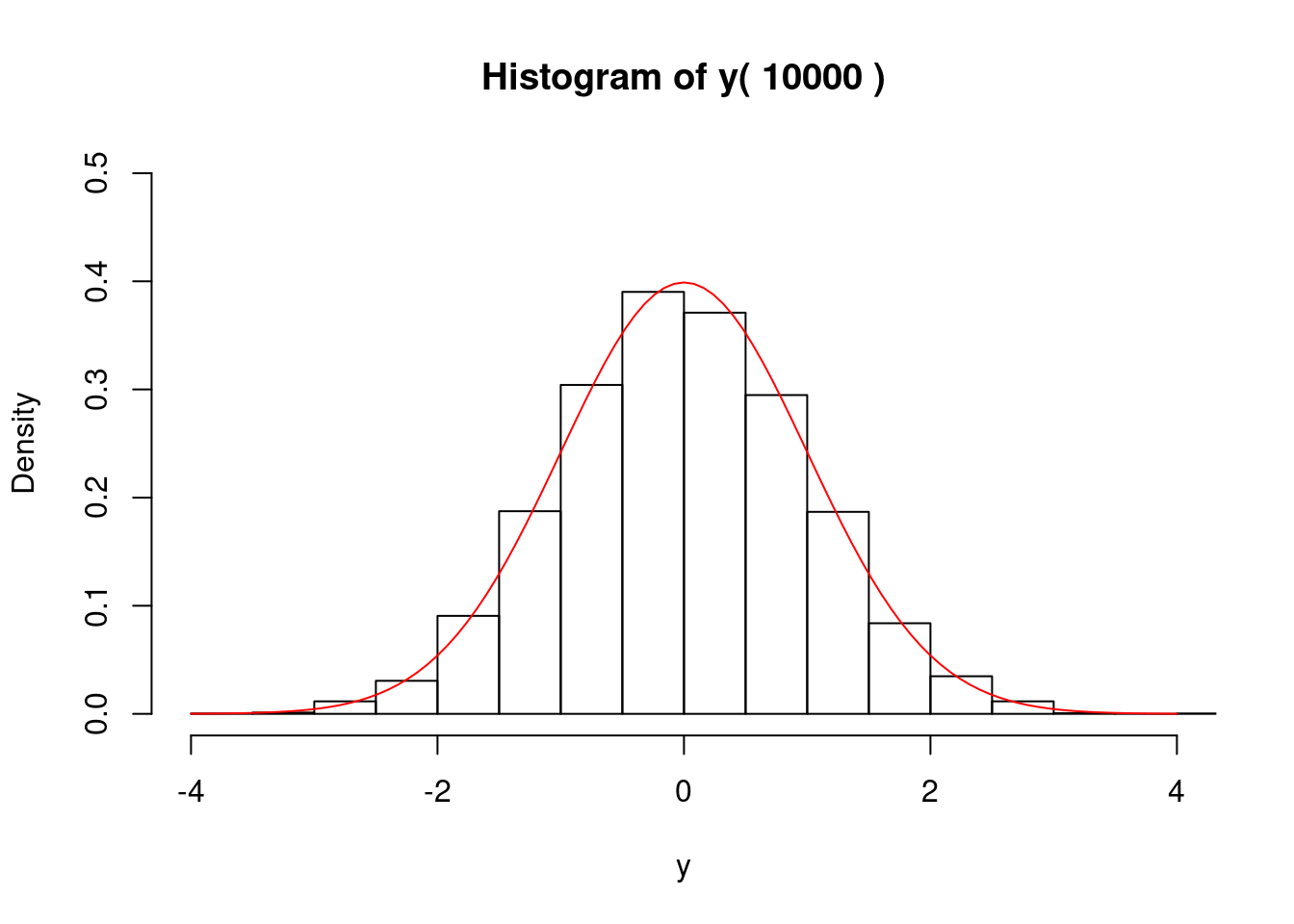
確率密度関数\(f(x)\)が\[ f(x) = \frac{1}{\sqrt{2\pi\sigma^2}}\, e^{- \frac{(x-\mu)^2}{2\sigma^2}} \quad (-\infty < x < \infty) \] で表せる確率分布を「平均\(\mu\),分散\(\sigma^2\)の正規分布」といい，\(X \sim {\rm N} (\mu, \,\sigma^2)\) と記す．特に\(\mu=0,\,\sigma^2=1^2\)のときの正規分布\({\rm N} (0, \,1^2)\)を標準正規分布という．以下では，標準正規分布に従う乱数(正規乱数)を中心刻限定理に基づいて生成する．

中心極限定理:
標本(確率変数)\(X_1,\cdots,X_s,\cdots,X_n\)が，互いに独立に同一の分布(平均\(\mu\)，分散\(\sigma^2\))に従うとき標本平均\(\bar{X} = \frac{1}{n}\,\sum_{s=1}^{n}\,X_s\)は，標本数\(n\)の増加に伴い，正規分布 \({\rm N}(\mu, \big(\frac{\sigma}{\sqrt{n}}\big)^2)\) に漸近する．

メモ： 総和\(T = \sum_{s=1}^{n}\,X_s\)は，正規分布 \({\rm N}(\mu, \big(\sqrt{n}\,\sigma \big)^2)\) に漸近する．また，確率変数\(X\)が区間\([a,b)\)上の一様分布に従うとき，\(X\)の平均\(\mu\)，分散\(\sigma^2\)はそれぞれ \(\mu = \frac{(a+b)}{2},~ \sigma^2 = \frac{(b-a)^2}{12}\)で表せる．

### 正規乱数
if (1) {
#  postscript("Rfig-3.eps",height=6,horizontal=F); 
#  par(mfrow=c(1,1),cex.main=1.5,cex.axis=1.5,lwd=1.5)
  set.seed(1)
  n <- 10000; n0 <- n*12 
  x <- runif(n0,-0.5,0.5) # 区間[-0.5,0.5)上の一様乱数を生成
  y <- rep(0,n)
  for (i in 1:n) {  # 12個づつの一様乱数の和を求める
    js <- 12*(i-1)+1; je <- 12*i; y[i] <- sum(x[js:je]) 
    }
  gmain <- paste("Histogram of y(",n,")")
  hist(y,freq=F,main=gmain,xlim=c(-4,4),ylim=c(0,0.5))
    curve(dnorm,-4,4,add=T,col="red")
#  graphics.off()
  }

乱数の応用

### 円の面積：モンテカルロ積分
if (1) {
#  postscript("Rfig-4.eps",height=9,horizontal=F); 
#  par(mfrow=c(1,1),pty="s",cex.main=1.5,cex.axis=1.5,lwd=1.5)
  par(pty="s")
  set.seed(1); n <- 1000;   x <- runif(n);   y <- runif(n)
  ic <- 0; xin <- c(); yin <- c(); xout <- c(); yout <- c()
  for (i in 1:n) {
    if (x[i]^2+y[i]^2 <= 1) 
       { ic <- ic + 1; xin <- c(xin,x[i]); yin <- c(yin,y[i])   }
    else { xout <- c(xout,x[i]); yout <- c(yout,y[i]) }
    } # end of for-i
  estpi <- ic/n * 4
  gmain <- paste("scatter plot of (x,y) n=",n," estpi=",estpi)
  plot(xout,yout,main=gmain,xlim=c(-0.2,1.2),ylim=c(-0.2,1.2))
    points(xin,yin,col="blue")
    curve(sqrt(1-x^2),0,1,add=T,col="red")
    grid(12,12)
#  graphics.off()
  } # end of if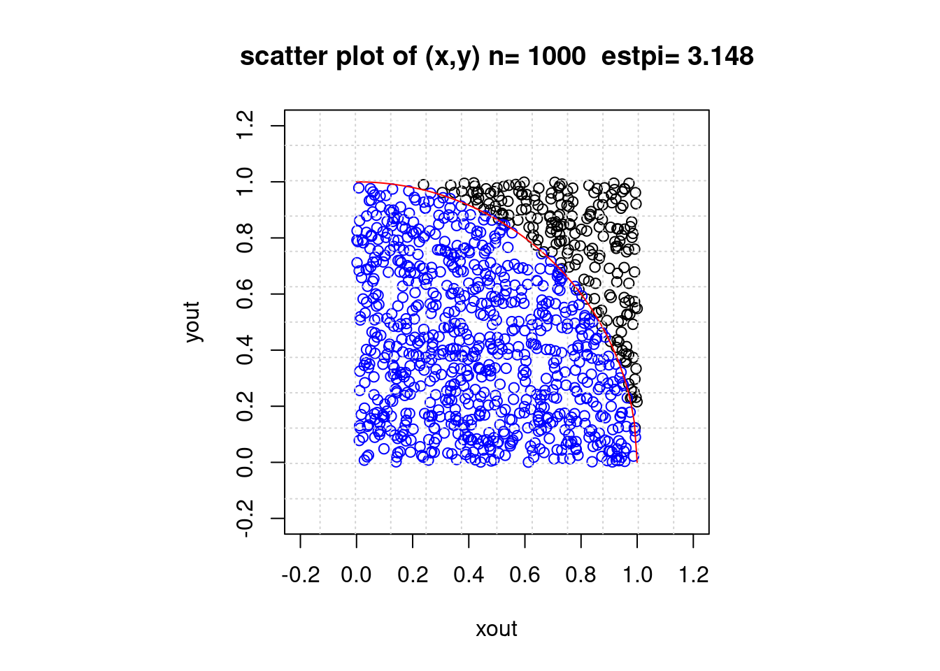

円の最小2乗法

データ \(\{(x_s, y_s), s=1,2,...,n\}\) に対して \(S = \sum_{s=1}^n \{(x_s-x_c)^2 + (y_s-y_c)^2 - r^2\}^2\) を最小にする円の中心座標 \((x_c, y_c)\) と半径 \(r\) を求める.

source("/home/inoue/r-ex/RLIB")
p <- c(xc<-2,yc<-3,r<-4) # (xc,yc,r)
cat("円の母数ベクトル: p=(xc,yc,r)=",p,"\n")

## 円の母数ベクトル: p=(xc,yc,r)= 2 3 4

cat("母数: xc=",xc,"yc=",yc,"r=",r,"\n")

## 母数: xc= 2 yc= 3 r= 4

n <- 50; ng <- 200; # n:データ数, ng:円表示点数, 
rate <- 3/4  # データの取得範囲を制限できる
t <- seq(0:(n-1))*2*pi/n*rate   # 半時計回りの角度 (0 <= t < 2*pi)
tg <- seq(0:(ng-1))*2*pi/ng     # 円を描画するための表示点の個数
xt <- xc + r*cos(t); xg <- xc + r*cos(tg)
yt <- yc + r*sin(t); yg <- yc + r*sin(tg)
### 誤差の生成
sd <- 0.5  # sd:誤差の標準偏差
  set.seed(1); xeps <- rnorm(n,0,sd=sd) # 正規乱数による誤差
  set.seed(2); yeps <- rnorm(n,0,sd=sd) # 正規乱数による誤差
### データの生成
x <- xt + xeps; y <- yt + yeps
### 母数変換 A=-2*xc, B= -2*yc, C=xc^2+yc^2-r^2 後の正規方程式 
M <- matrix(0,nrow=3,ncol=3)
M[1,] <- c(sum(x^2), sum(x*y), sum(x))
M[2,] <- c(sum(y*x), sum(y^2), sum(y))
M[3,] <- c(sum(1*x), sum(1*y),   n)
b <- c(-sum((x^2+y^2)*x), -sum((x^2+y^2)*y), -sum((x^2+y^2)*1))
ans <- solve(M,b)  # 正規方程式を解く
cat("解ベクトル: ans=",ans," (<- 母数変換された解ベクトル)\n")

## 解ベクトル: ans= -3.931338 -6.287147 -3.196632  (<- 母数変換された解ベクトル)

### 母数逆変換 ans=(A,B,C) -> ph=(xch,ych,rh) 
ph <- c(-0.5*ans[1], -0.5*ans[2], sqrt(0.25*ans[1]^2+0.25*ans[2]^2-ans[3]))
cat("推定解ベクトル: ph=",ph,"\n")

## 推定解ベクトル: ph= 1.965669 3.143574 4.116132

xh <- ph[1] + ph[3]*cos(tg)
yh <- ph[2] + ph[3]*sin(tg)
### 描画
#g.on("fig-1")
par(pty="s",cex=0.75)
plot(x,y,xlim=c(xc-1.5*r,xc+1.5*r),ylim=c(yc-1.5*r,yc+1.5*r))
main <- "true circle(blue) and estimated circle(red)"
sub <- paste("\n true: (xc, yc, r)=(",p[1],", ",p[2],", ",p[3], 
             "),  n=",n, ", sd=",sd,", rate=",round(rate,3),"\n", 
             "est.: (xch, ych, rh)=(",
              round(ph[1],3),", ",round(ph[2],3),", ",round(ph[3],3),")")
title(main=main,sub=sub)
### 真円描画
xg <- c(xg,xg[1]); yg <- c(yg,yg[1])
par(new=T)
plot(xg,yg,type="l",col="blue",xlab="",ylab="",
     xlim=c(xc-1.5*r,xc+1.5*r),ylim=c(yc-1.5*r,yc+1.5*r))
points(p[1],p[2],col="blue",pch=3)
### 推定円描画
par(new=T)
xh <- c(xh,xh[1]); yh <- c(yh,yh[1])
plot(xh,yh,type="l",col="red",xlab="",ylab="",
     ,xlim=c(xc-1.5*r,xc+1.5*r),ylim=c(yc-1.5*r,yc+1.5*r))
points(ph[1],ph[2],col="red",pch=3)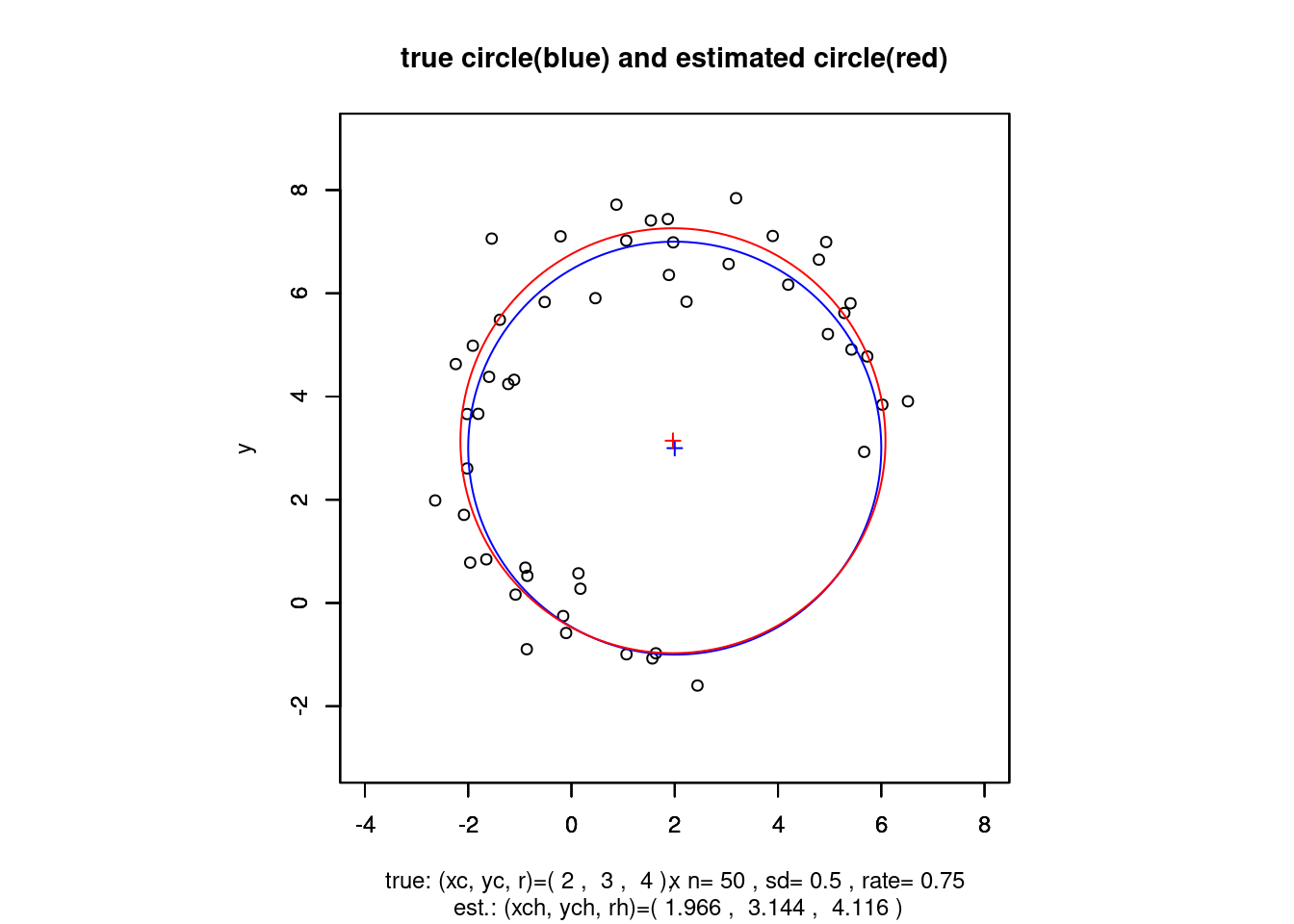

#g.off(); g.view("fig-1");q()

球の最小2乗法

データ \(\{(x_s, y_s, z_s), s=1,2,...,n\}\) に対して \(S = \sum_{s=1}^n \{(x_s-x_c)^2 + (y_s-y_c)^2 + (z_s-z_c)^2 - r^2\}^2\) を最小にする球の中心座標 \((x_c, y_c, z_c)\) と半径\(r\)を求める.

source("/home/inoue/r-ex/RLIB")
p <- c(xc<-1,yc<-2,zc<-3,r<-4) # (xc,yc,zc,r)
cat("球の母数ベクトル:　p=(xc,yc,zc,r)=",p,"\n")

## 球の母数ベクトル:　p=(xc,yc,zc,r)= 1 2 3 4

cat("母数:　xc=",xc,"yc=",yc,"zc=",zc,"r=",r,"\n")

## 母数:　xc= 1 yc= 2 zc= 3 r= 4

#　nt: 緯度方向のデータ数, nu: 経度方向のデータ数, n=nt*nu:データ数
nt <- 10; nu <- 20; n <- nt*nu         # 0 <= t < pi, 0 <= u < 2*pi
rate <- 1　#　緯度，経度に関するデータ取得率
t <- seq(0:(nt-1))*pi/nt   * rate  
u <- seq(0:(nu-1))*2*pi/nu * rate 
### データ点を作成する
xt <- rep(0,n); yt <- rep(0,n); zt <- rep(0,n)
for (i in 1:nt) { 
   for (j in 1:nu) {
     xt[nu*(i-1)+j] <- xc + r*sin(t[i])*cos(u[j]) 
     yt[nu*(i-1)+j] <- yc + r*sin(t[i])*sin(u[j])
     zt[nu*(i-1)+j] <- zc + r*cos(t[i])
     }
    }
sd <- 0.5  # sd:誤差の標準偏差
  set.seed(1); xeps <- rnorm(n,0,sd=sd)　　#　正規乱数による誤差
  set.seed(2); yeps <- rnorm(n,0,sd=sd)　　#　正規乱数による誤差
  set.seed(3); zeps <- rnorm(n,0,sd=sd)　　#　正規乱数による誤差
### 誤差を伴ったデータベクトル x, y, z (n*1) を生成する
x <- xt + xeps; y <- yt + yeps; z <- zt + zeps
### 描画用作図点を作成する
ngt <- 30; ngu <- 60; ng <- (ngt+1)*(ngu+1)
tg <- seq(0:ngt)*pi/ngt　　　　#　球を描画するための表示点の個数(緯度方向)
ug <- seq(0:ngu)*2*pi/ngu　　#　球を描画するための表示点の個数(経度方向)
### 母数変換 A=-2*xc, B= -2*yc, C = -2*zc, D=xc^2+yc^2+zc^2-r^2　後の正規方程式 
M <- matrix(0,nrow=4,ncol=4)
M[1,] <- c(sum(x^2), sum(x*y), sum(x*z), sum(x*1))
M[2,] <- c(sum(y*x), sum(y^2), sum(y*z), sum(y*1))
M[3,] <- c(sum(z*x), sum(z*y), sum(z^2), sum(z*1))
M[4,] <- c(sum(1*x), sum(1*y), sum(1*z),    n)
b <- c(-sum((x^2+y^2+z^2)*x), -sum((x^2+y^2+z^2)*y), 
       -sum((x^2+y^2+z^2)*z), -sum((x^2+y^2+z^2)*1))
ans <- solve(M,b)  # 正規方程式を解く
cat("解ベクトル:　ans=",ans," (<- 母数変換された解ベクトル)\n")

## 解ベクトル:　ans= -2.188196 -3.966385 -5.944339 -2.380663  (<- 母数変換された解ベクトル)

### 母数逆変換 ans=(A,B,C,D) -> ph=(xch,ych,zch,rh) 
ph <- c(-0.5*ans[1], -0.5*ans[2], -0.5*ans[3],
        sqrt(0.25*ans[1]^2+0.25*ans[2]^2+0.25*ans[3]^2-ans[4]))
cat("推定解ベクトル:　ph=",ph,"\n")

## 推定解ベクトル:　ph= 1.094098 1.983193 2.972169 4.04284

### 推定された球の(x,y,z)座標
xh <- rep(0,ng); yh <- rep(0,ng); zh <- rep(0,ng)
for (i in 1:(ngt+1)) { 
   for (j in 1:(ngu+1)) {
     xh[(ngu+1)*(i-1)+j] <- ph[1] + ph[4]*sin(tg[i])*cos(ug[j]) 
     yh[(ngu+1)*(i-1)+j] <- ph[2] + ph[4]*sin(tg[i])*sin(ug[j])
     zh[(ngu+1)*(i-1)+j] <- ph[3] + ph[4]*cos(tg[i])
     }
    }
### 真球の(x,y,z)座標
xg <- rep(0,ng); yg <- rep(0,ng); zg <- rep(0,ng)
for (i in 1:(ngt+1)) { 
   for (j in 1:(ngu+1)) {
     xg[(ngu+1)*(i-1)+j] <- xc + r*sin(tg[i])*cos(ug[j]) 
     yg[(ngu+1)*(i-1)+j] <- yc + r*sin(tg[i])*sin(ug[j])
     zg[(ngu+1)*(i-1)+j] <- zc + r*cos(tg[i])
     }
    }
#g.on("fig-2",height=27)
library(scatterplot3d)
par(mfrow=c(3,1),cex=0.7,pty="s")  # pty="s"
scatterplot3d(x,y,z,
        xlim=c(xc-1.5*r,xc+1.5*r),ylim=c(yc-1.5*r,yc+1.5*r),
        zlim=c(zc-1.5*r,zc+1.5*r))
main=paste("Data: (x_s, y_s, z_s), s=1, 2, ..., n, where n=", n)
title(main=main)
### 真球描画
scatterplot3d(xg,yg,zg,highlight.3d=T,col.grid="blue",
     xlim=c(xc-1.5*r,xc+1.5*r),ylim=c(yc-1.5*r,yc+1.5*r),
     zlim=c(zc-1.5*r,zc+1.5*r))
main <- paste("True Sphere (xc=",p[1],", yc=",p[2],", zc=",p[3],", r=",p[4],")")
title(main=main)
###　推定球描画
scatterplot3d(xh,yh,zh,highlight.3d=T,
     xlim=c(xc-1.5*r,xc+1.5*r),ylim=c(yc-1.5*r,yc+1.5*r),
     zlim=c(zc-1.5*r,zc+1.5*r))
main <- paste("Estimated Sphere (xc=",round(ph[1],3),
              ", yc=",round(ph[2],3),", zc=",round(ph[3],3),
              ", r=",round(ph[4],3),")")
title(main=main)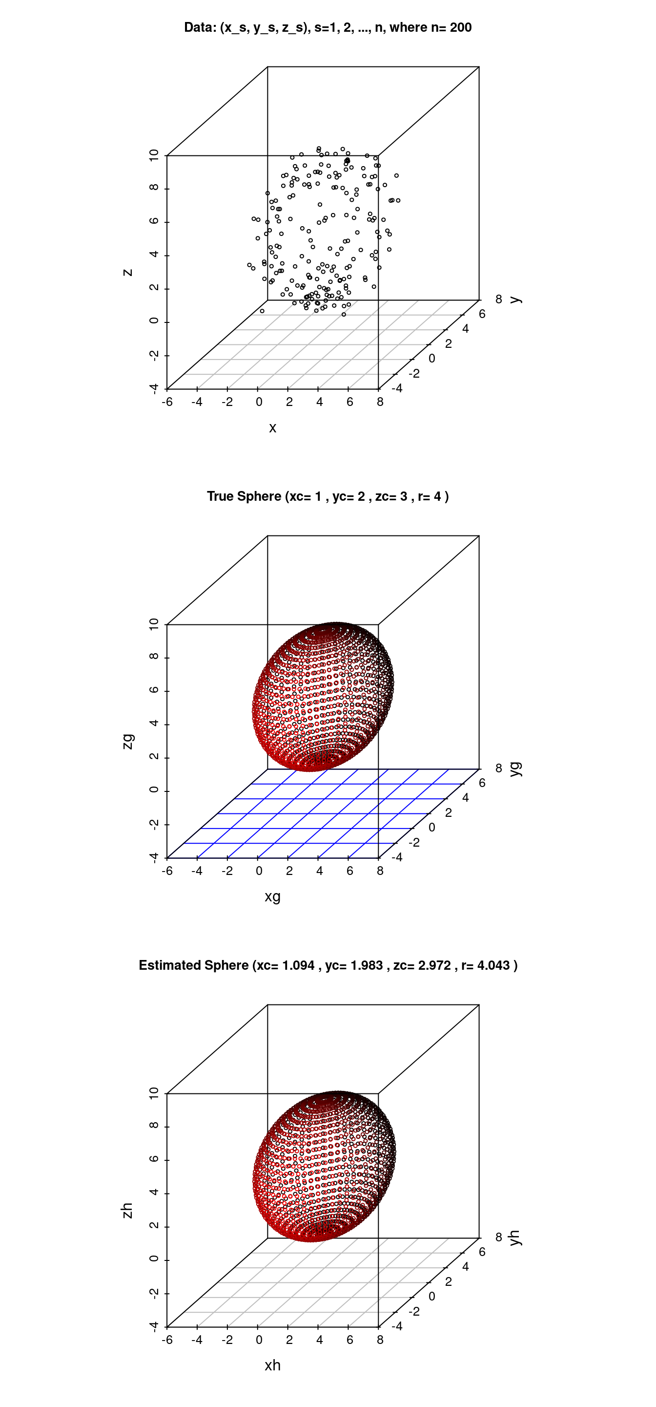

R言語私用ライブラリRLIBのメモ: ex-persp.Rnw

関数 persp() の定義

methods(persp)

## [1] persp.default*
## see '?methods' for accessing help and source code

getS3method("persp","default")

## function (x = seq(0, 1, length.out = nrow(z)), y = seq(0, 1, 
##     length.out = ncol(z)), z, xlim = range(x), ylim = range(y), 
##     zlim = range(z, na.rm = TRUE), xlab = NULL, ylab = NULL, 
##     zlab = NULL, main = NULL, sub = NULL, theta = 0, phi = 15, 
##     r = sqrt(3), d = 1, scale = TRUE, expand = 1, col = "white", 
##     border = NULL, ltheta = -135, lphi = 0, shade = NA, box = TRUE, 
##     axes = TRUE, nticks = 5, ticktype = "simple", ...) 
## {
##     if (is.null(xlab)) 
##         xlab <- if (!missing(x)) 
##             deparse(substitute(x))
##         else "X"
##     if (is.null(ylab)) 
##         ylab <- if (!missing(y)) 
##             deparse(substitute(y))
##         else "Y"
##     if (is.null(zlab)) 
##         zlab <- if (!missing(z)) 
##             deparse(substitute(z))
##         else "Z"
##     if (missing(z)) {
##         if (!missing(x)) {
##             if (is.list(x)) {
##                 z <- x$z
##                 y <- x$y
##                 x <- x$x
##             }
##             else {
##                 z <- x
##                 x <- seq.int(0, 1, length.out = nrow(z))
##             }
##         }
##         else stop("no 'z' matrix specified")
##     }
##     else if (is.list(x)) {
##         y <- x$y
##         x <- x$x
##     }
##     if (any(diff(x) <= 0) || any(diff(y) <= 0)) 
##         stop("increasing 'x' and 'y' values expected")
##     if (box) {
##         zz <- z[!is.na(z)]
##         if (any(x < xlim[1]) || any(x > xlim[2]) || any(y < ylim[1]) || 
##             any(y > ylim[2]) || any(zz < zlim[1]) || any(zz > 
##             zlim[2])) 
##             warning("surface extends beyond the box")
##     }
##     ticktype <- pmatch(ticktype, c("simple", "detailed"))
##     plot.new()
##     r <- .External.graphics(C_persp, x, y, z, xlim, ylim, zlim, 
##         theta, phi, r, d, scale, expand, col, border, ltheta, 
##         lphi, shade, box, axes, nticks, ticktype, as.character(xlab), 
##         as.character(ylab), as.character(zlab), ...)
##     for (fun in getHook("persp")) {
##         if (is.character(fun)) 
##             fun <- get(fun)
##         try(fun())
##     }
##     if (!is.null(main) || !is.null(sub)) 
##         title(main = main, sub = sub, ...)
##     invisible(r)
## }
## <bytecode: 0x562e8121de08>
## <environment: namespace:graphics>

require(grDevices) # for trans3d
trans3d　　　　　　　　　　　　　　　　# trans3d　の定義

## function (x, y, z, pmat) 
## {
##     tr <- cbind(x, y, z, 1, deparse.level = 0L) %*% pmat
##     list(x = tr[, 1]/tr[, 4], y = tr[, 2]/tr[, 4])
## }
## <bytecode: 0x562e810d2e78>
## <environment: namespace:grDevices>

#getS3method("trans3d","graphics")

使用例

require(grDevices) # for trans3d
     ## More examples in  demo(persp) !!
     ##                   -----------
     # (1) The Obligatory Mathematical surface.
     #     Rotated sinc function.
     
     x <- seq(-10, 10, length= 30)
     y <- x
     f <- function(x, y) { r <- sqrt(x^2+y^2); 10 * sin(r)/r }
     z <- outer(x, y, f)
     z[is.na(z)] <- 1
     op <- par(bg = "white")
     persp(x, y, z, theta = 30, phi = 30, expand = 0.5, col = "lightblue")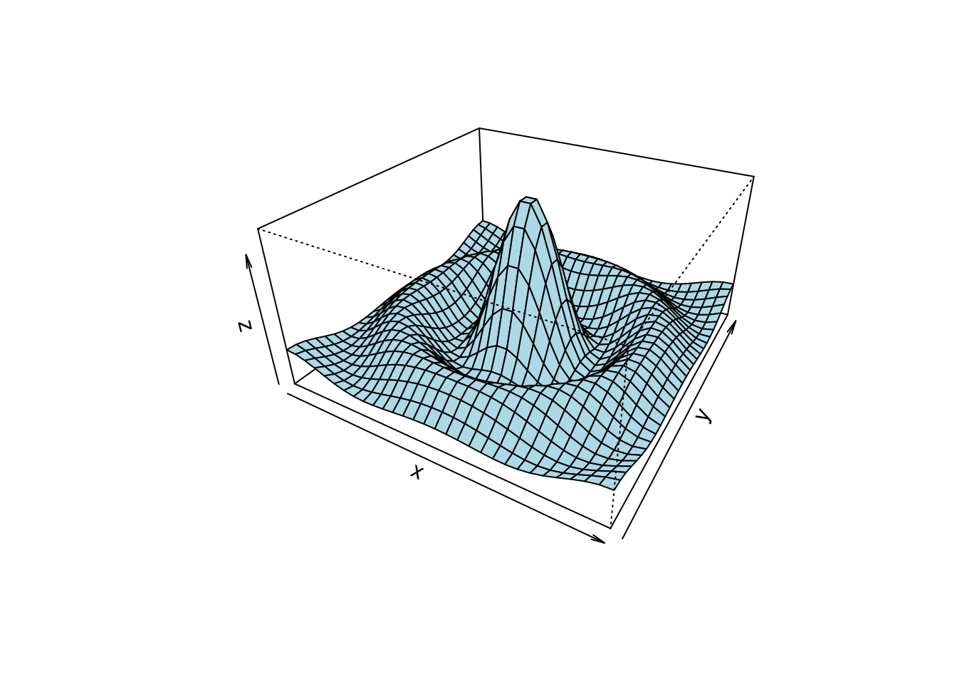

     # 第２図
     persp(x, y, z, theta = 30, phi = 30, expand = 0.5, col = "lightblue",
           ltheta = 120, shade = 0.75, ticktype = "detailed",
           xlab = "X", ylab = "Y", zlab = "Sinc( r )"
     ) -> res
     round(res, 3)

##       [,1]   [,2]   [,3]   [,4]
## [1,] 0.087 -0.025  0.043 -0.043
## [2,] 0.050  0.043 -0.075  0.075
## [3,] 0.000  0.074  0.042 -0.042
## [4,] 0.000 -0.273 -2.890  3.890

     # (2) Add to existing persp plot - using trans3d() :
     xE <- c(-10,10); xy <- expand.grid(xE, xE)
     ### 4隅に赤点をプロット
     points(trans3d(xy[,1], xy[,2], 6, pmat = res), col = 2, pch = 16)
     ### 側面(y=10)に緑のサインカーブを追加描画
     lines (trans3d(x, y = 10, z = 6 + sin(x), pmat = res), col = 3)
     ### 第2最大値をとる曲線をピンクで描画(等高線描画)
     phi <- seq(0, 2*pi, len = 201)
     r1 <- 7.725 # radius of 2nd maximum
     xr <- r1 * cos(phi)
     yr <- r1 * sin(phi)
     lines(trans3d(xr,yr, f(xr,yr), res), col = "pink", lwd = 2)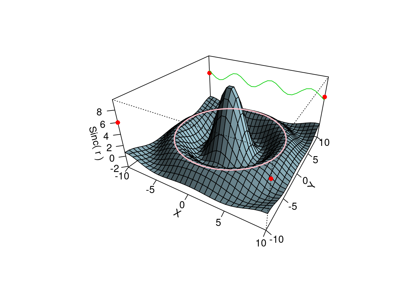

     ## (no hidden lines)

     # (3) Visualizing a simple DEM model
     
     z <- 2 * volcano        # Exaggerate the relief
     x <- 10 * (1:nrow(z))   # 10 meter spacing (S to N)
     y <- 10 * (1:ncol(z))   # 10 meter spacing (E to W)
     ## Don't draw the grid lines :  border = NA
     par(bg = "slategray")
     persp(x, y, z, theta = 135, phi = 30, col = "green3", scale = FALSE,
           ltheta = -120, shade = 0.75, border = NA, box = FALSE)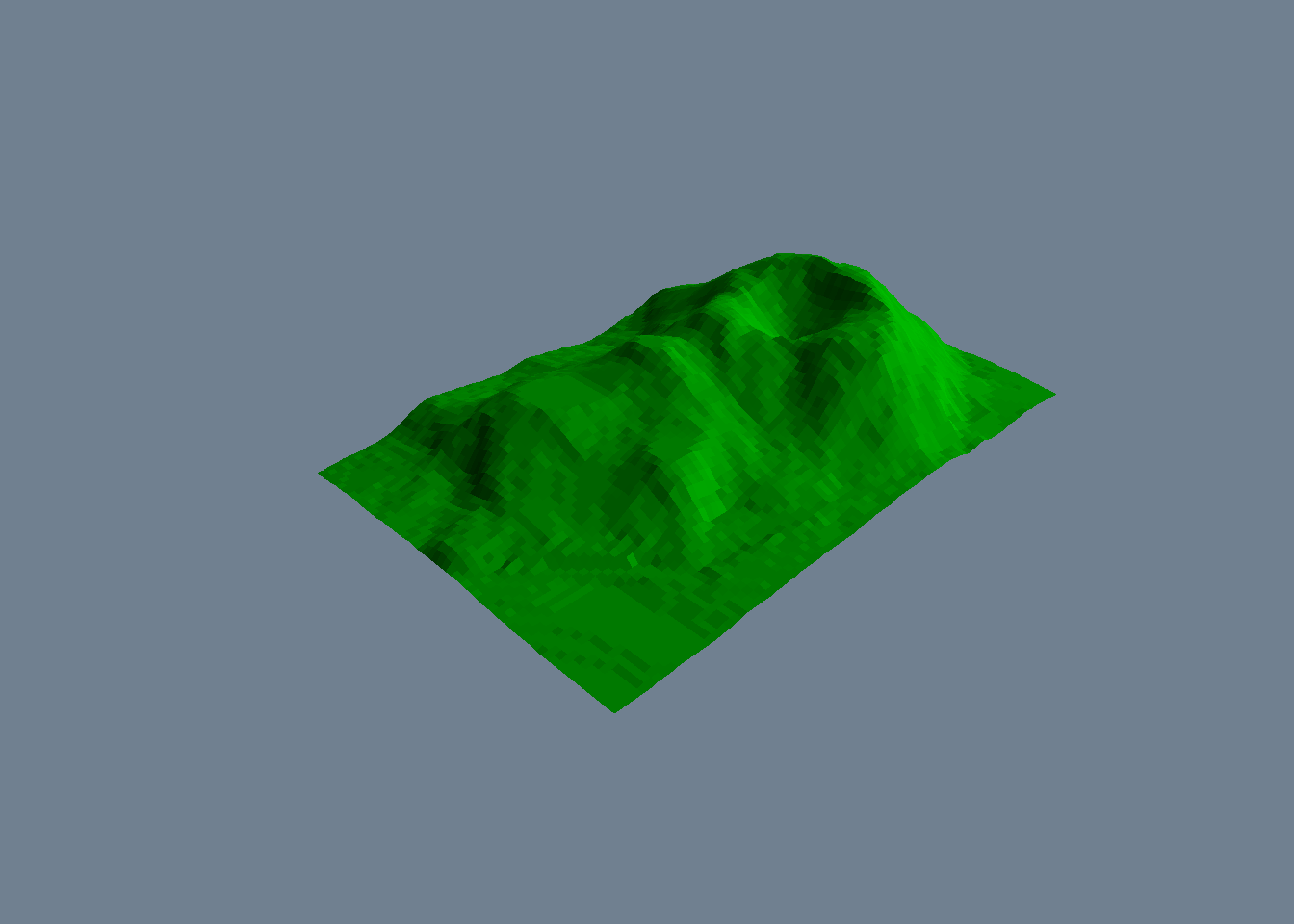

     # (4) Surface colours corresponding to z-values
     
     par(bg = "white")
     x <- seq(-1.95, 1.95, length = 30)
     y <- seq(-1.95, 1.95, length = 35)
     z <- outer(x, y, function(a, b) a*b^2)
     nrz <- nrow(z)
     ncz <- ncol(z)
     # Create a function interpolating colors in the range of specified colors
     jet.colors <- colorRampPalette( c("blue", "green") )
     # Generate the desired number of colors from this palette
     nbcol <- 100
     color <- jet.colors(nbcol)
     # Compute the z-value at the facet centres
     zfacet <- z[-1, -1] + z[-1, -ncz] + z[-nrz, -1] + z[-nrz, -ncz]
     # Recode facet z-values into color indices
     facetcol <- cut(zfacet, nbcol)
     persp(x, y, z, col = color[facetcol], phi = 30, theta = -30)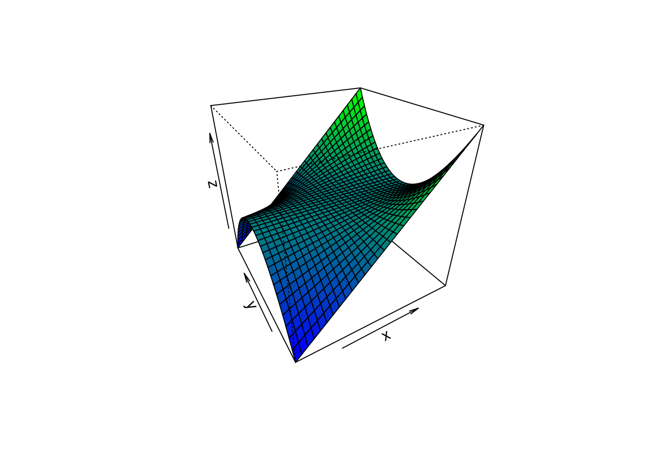

     par(op)

2変量正規分布と条件付き分布，周辺分布

### plot3func 2変数関数の鳥瞰図，等高線図の作図 #############
plot3func <- function(xlim,ylim,func,contour=T,...){
  gx <- seq(xlim[1],xlim[2],length=51)
  gy <- seq(ylim[1],ylim[2],length=51)
  gz <- outer(gx,gy, func)
  op <- par(no.readonly=TRUE)
  if (contour) {
     mat <- matrix(c(1,1,1,0,0,  1,1,1,2,2,  1,1,1,2,2, 
                     1,1,1,2,2,  1,1,1,0,0), ncol=5, byrow=T)
     layout(mat)  
     }
  persp(gx, gy, gz, xlim=xlim, ylim=ylim,
        xlab="x", ylab="y", zlab="Dens.",
        theta=30, phi=30, 
        ticktype="detailed", nticks=3, 
        expand=0.5, shade=0.5, col="cyan",...)
  if (contour) {
      par(pty="s") 
     gx <- seq(xlim[1],xlim[2],length=101)
     gy <- seq(ylim[1],ylim[2],length=101)
     gz <- outer(gx,gy, func)
     #  levels <- seq(0, max(gz)*0.7,length=7)
     #   contour(gx, gy, gz, xlab="x", ylab="y",levels=levels)
        image(gx, gy, gz, xlab="x", ylab="y",
              col =  c("gray", heat.colors(12)) )
     }
 par(op)
}

##########################################
func.xy <- function(x,y){ # 2変量度数分布表から同時密度関数を生成
   f <- rep(0, length(x)); ie <- length(xbrk)-1; je <- length(ybrk)-1
   for (i in 1:ie) {
     for (j in 1:je) {
       fx <- -1*(x-xbrk[i])*(x-xbrk[i+1]); fx <- round(fx,3);
       fy <- -1*(y-ybrk[j])*(y-ybrk[j+1]); fy <- round(fy,3)
       # cat("fun: fx", fx, "\n")
       for (s in 1:length(x)) {
         if ( (fx[s] >= 0)  & (fy[s] >= 0) )  { 
           f[s] <- fxy[i,j]/(xbrk[i+1]-xbrk[i])/(ybrk[j+1]-ybrk[j]) }
         } #  end of for-s
       } # end of for-j
   } # end of for-i
   #cat("fun: z ",f,"\n")
   return(f)
   } # end of fun

### dnorm2 : ２変量正規分布の密度関数
dnorm2 <- function(x, y, means=c(0,0), sds=c(1,1), cor=0){
  mux <- means[1]; sdx <- sds[1]
  muy <- means[2]; sdy <- sds[2]
   #cat("func: x ",x,"\n")
   #cat("func: y ",y,"\n")
  f1 <- 2*pi *  sdx * sdy * sqrt(1-cor^2)
  f2 <- ((x-mux)/sdx)^2 - 2*cor*((x-mux)/sdx)*((y-muy)/sdy) + ((y-muy)/sdy)^2
  f2 <- exp(-0.5 / (1-cor^2) * f2)
  f <- f2/f1
  #cat("func: z ",f,"\n")
  return(f)
}

###### main #########################################################
require(grDevices)
par(family="Japan1",mfrow=c(1,1))
cor <- 0.7
f <- function(x,y){ dnorm2(x,y,means=c(0,0),sds=c(1,1),cor=cor)}
x <- seq(-4,4,length=51)
y <- seq(-4,4,length=51)
z <- outer(x,y,f); z[is.na(z)] <- 0;
### 同時密度関数 z=f(x,y)
xlim <- range(x); ylim <- range(y); zlim <- c(min(z), max(z)*1.05)
plot3func(xlim,ylim,f,contour=T) ### 私用関数による描画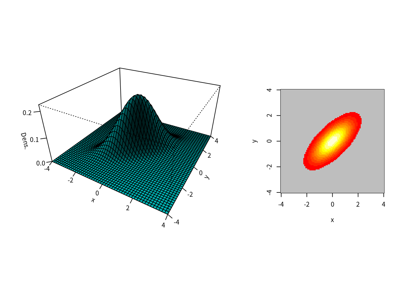

op <- par(bg="white",family="Japan1")
main <- "同時密度関数: f(x,y)"
res <- persp(x,y,z,theta=30,phi=30,expand=0.5,col="lightblue",
      ltheta=120,shade=0.75,ticktype="detailed",
      xlim=xlim,ylim=ylim,zlim=zlim,main=main,
      xlab="x",ylab="y",zlab="f(x,y)") 
round(res,3)   ### 3次元データ(x,y,z)を平面に投影する情報をresに保存

##       [,1]   [,2]   [,3]   [,4]
## [1,] 0.217 -0.062  0.108 -0.108
## [2,] 0.125  0.108 -0.188  0.188
## [3,] 0.000  3.701  2.137 -2.137
## [4,] 0.000 -0.433 -2.982  3.982

### 切断面を描画　(pmat=res で使用）
x0 <- 1; y0 <- -1; zmin <- min(z); zmax <- max(z)
lines(trans3d(x,y=y0,z=f(x,y0),pmat=res),col="red",lwd=2)
  lines(trans3d(x,y=y0,z=0,pmat=res),col="red",lwd=1)
  lines(trans3d(x,y=y0,z=zmax,pmat=res),col="red",lwd=1)
  lines(trans3d(x=xlim[1],y=y0,z=c(zmin,zmax),pmat=res),col="red",lwd=1)
  lines(trans3d(x=xlim[2],y=y0,z=c(zmin,zmax),pmat=res),col="red",lwd=1)
lines(trans3d(x=x0,y,z=f(x0,y),pmat=res),col="blue",lwd=2)
  lines(trans3d(x=x0,y,z=0,pmat=res),col="blue",lwd=1)
  lines(trans3d(x=x0,y,z=zmax,pmat=res),col="blue",lwd=1)
  lines(trans3d(x=x0,y=ylim[1],z=c(zmin,zmax),pmat=res),col="blue",lwd=1)
  lines(trans3d(x=x0,y=ylim[2],z=c(zmin,zmax),pmat=res),col="blue",lwd=1)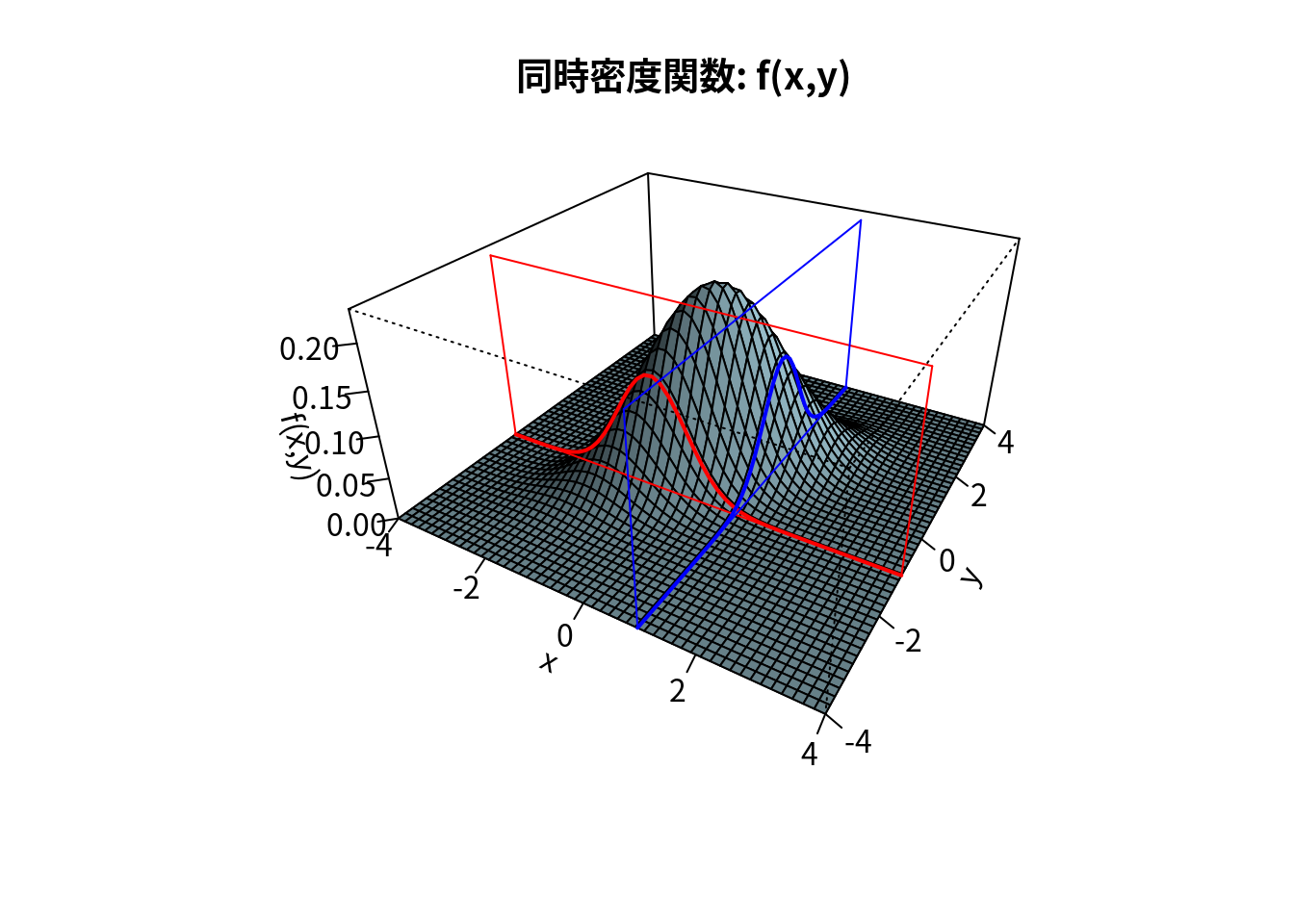

######################
x <- seq(-4,4,length=51)
y <- seq(-4,4,length=51)
f0 <- function(x,y) { x+y-x-y }
z <- outer(x,y,f); z[is.na(z)] <- 0; 
xlim <- range(x); ylim <- range(y); 
op <- par(bg="white",family="Japan1")
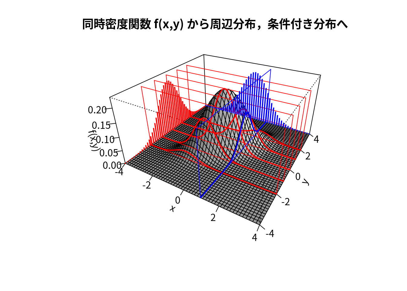
main <- "同時密度関数 f(x,y) から周辺分布，条件付き分布へ"
res <- persp(x,y,z,theta=30,phi=30,expand=0.5,col="white",
      ltheta=120,shade=0.75,ticktype="detailed",
      xlim=xlim,ylim=ylim,zlim=zlim,main=main,
      xlab="x",ylab="y",zlab="f(x,y)") 
round(res,3)

##       [,1]   [,2]   [,3]   [,4]
## [1,] 0.217 -0.062  0.108 -0.108
## [2,] 0.125  0.108 -0.188  0.188
## [3,] 0.000  3.701  2.137 -2.137
## [4,] 0.000 -0.433 -2.982  3.982

for (y0 in c(-2,-1,0,1,2)) { ### y=y0 での切断面を描画
  lines(trans3d(x,y=y0,z=f(x,y0),pmat=res),col="red",lwd=2)
    lines(trans3d(x,y=y0,z=0,pmat=res),col="red",lwd=1)
    lines(trans3d(x,y=y0,z=zmax,pmat=res),col="red",lwd=1)
    lines(trans3d(x=xlim[1],y=y0,z=c(zmin,zmax),pmat=res),col="red",lwd=1)
    lines(trans3d(x=xlim[2],y=y0,z=c(zmin,zmax),pmat=res),col="red",lwd=1)
  }
for (y0 in y) { ### y側面にｙ周辺分布のイメージを描画
  fx <- function(x){f(x,y=y0)}
  integ <- integrate(fx, -4,4); v <- integ$value/2   # 
  lines(trans3d(x=xlim[1],y=y0,z=c(zmin,v),pmat=res),col="red",lwd=2)
  }

for (x0 in c(1)) { ### x=x0 での切断面を描画
  lines(trans3d(x=x0,y,z=f(x0,y),pmat=res),col="blue",lwd=2)
    lines(trans3d(x=x0,y,z=0,pmat=res),col="blue",lwd=1)
    lines(trans3d(x=x0,y,z=zmax,pmat=res),col="blue",lwd=1)
    lines(trans3d(x=x0,y=ylim[1],z=c(zmin,zmax),pmat=res),col="blue",lwd=1)
    lines(trans3d(x=x0,y=ylim[2],z=c(zmin,zmax),pmat=res),col="blue",lwd=1)
  }
for (x0 in x) { ### x側面にx周辺分布のイメージを描画
  fy <- function(y){f(x=x0,y)}
  integ <- integrate(fy, -4,4); v <- integ$value/2
  lines(trans3d(x=x0,y=ylim[2],z=c(zmin,v),pmat=res),col="blue",lwd=2)
  }

####### 切断面関数の2次元描画
x0 <- 1; y0 <- -2; par(mfrow=c(2,2),family="Japan1")
x <- seq(-4,4,length=100); zx <- f(x,y=y0)
main <- paste("切断面関数：f(x,y=",y0,")")
plot(x,zx,ylim=zlim,type="l",col="red",ylab="",main=main)
y <- seq(-4,4,length=100); zy <- f(x=x0,y)
main <- paste("切断面関数 : f(x=",x0,",y)")
plot(y,zy,ylim=zlim,type="l",col="blue",ylab="",main=main)
### 条件付き密度関数
fx <- function(x){f(x,y=y0)}
integ <- integrate(fx, -4,4); zx0 <- integ$value 
main <- paste("条件付き密度関数：f(x|y=",y0,")")
plot(x,zx/zx0,ylim=c(0,0.7),type="l",col="red",ylab="",main=main)

fy <- function(y){f(x=x0,y)}
integ <- integrate(fy, -4,4); zy0 <- integ$value 
main <- paste("条件付き密度関数：f(y|x=",x0,")")
plot(y,zy/zy0,ylim=c(0,0.7),type="l",col="blue",ylab="",main=main)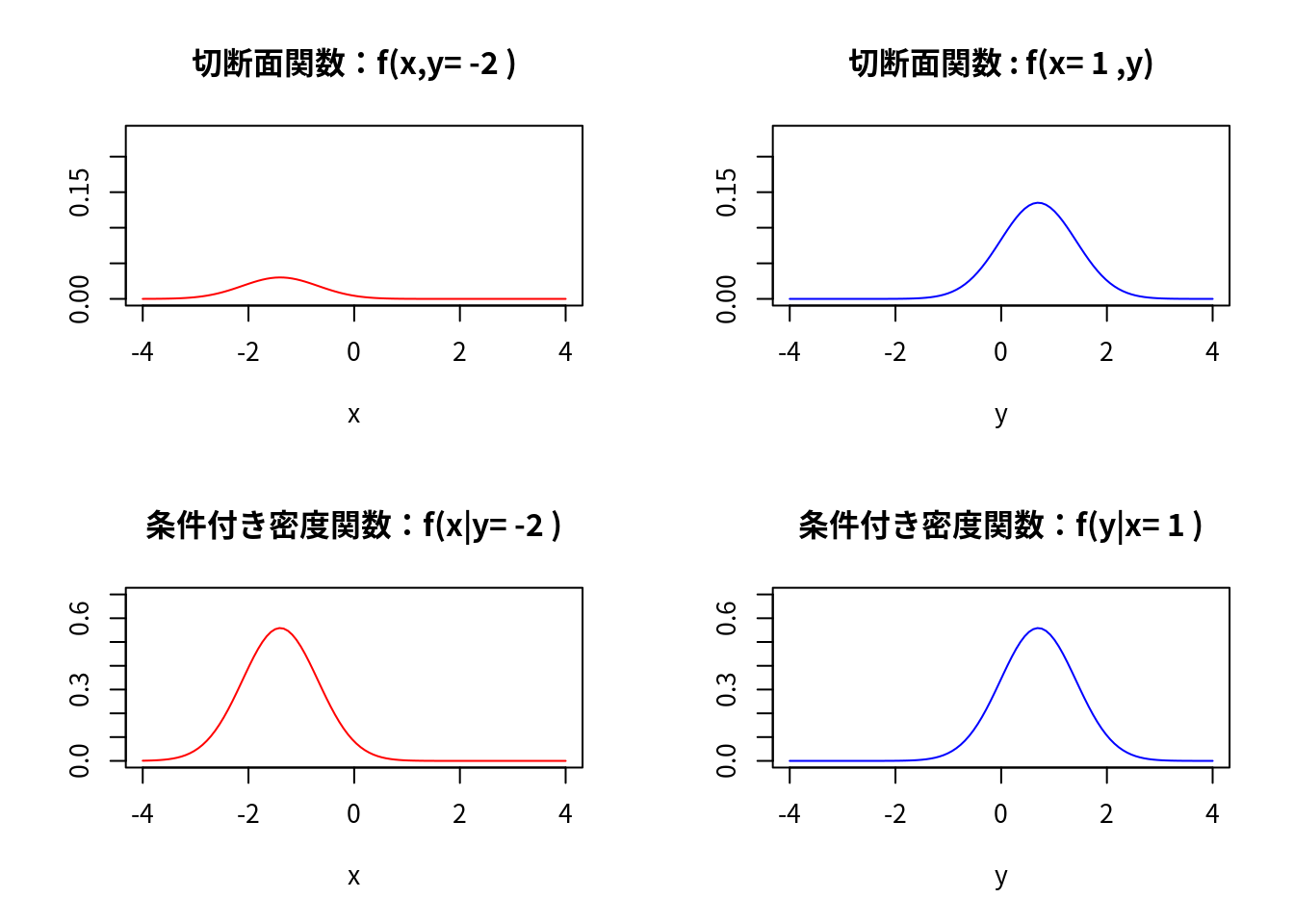

par(mfrow=c(1,2),family="Japan1")
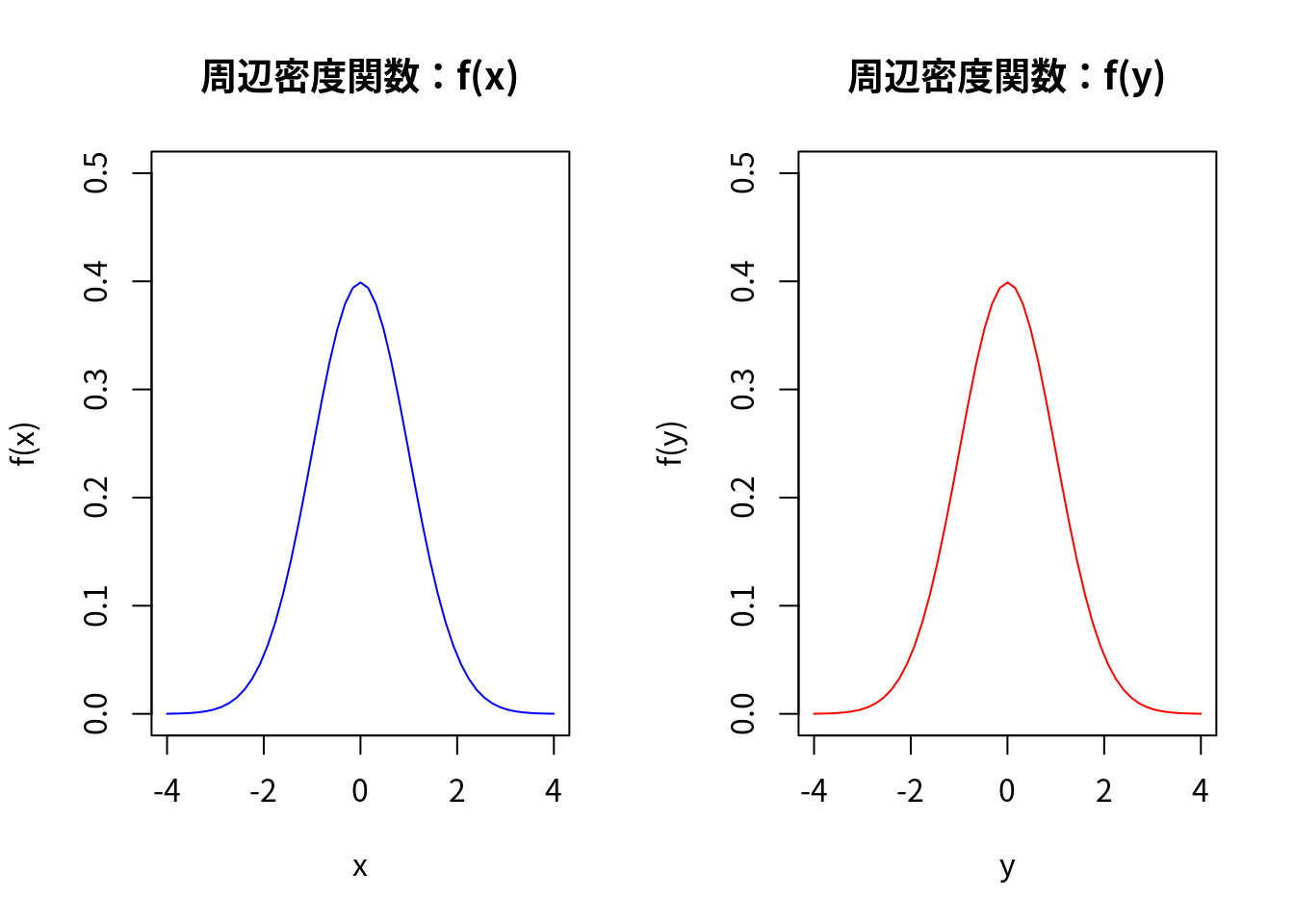
### 周辺密度関数 f(x) の描画
vx <- seq(-4,4,length=51); vf <- rep(0,51)
for (i in 1:length(vx)) {
  fy <- function(y){f(x=vx[i],y)};
  integ <- integrate(fy, -4,4); vf[i] <- integ$value
  }

main <- "周辺密度関数：f(x)"
plot(vx,vf,type="l",xlab="x",ylab="f(x)",ylim=c(0,0.5),col="blue",main=main)
### 周辺密度関数 f(y) の描画
vy <- seq(-4,4,length=51); vf <- rep(0,51)
for (i in 1:length(vy)) {
  fx <- function(x){f(x,y=vy[i])}
  integ <- integrate(fx, -4,4); vf[i] <- integ$value
  }
main <- "周辺密度関数：f(y)"
plot(vy,vf,type="l",xlab="y",ylab="f(y)",ylim=c(0,0.5),col="red",main=main)